
Paws and Reflect: Which Dog Should I Select?
Published:

Executive Summary
Paws-ing and Reflecting on Selecting a Dog? The Solution is Here for You
As an aspiring dog owner paws-es and reflects on which dog he/she should select, the team developed a solution to find the intelligent match between an aspiring dog owner and the dog that best fits his/her lifestyle and preferences.
Dimensionality Reduction and Information Retrieval Pipeline
To go about the solution, the team performed the following:
1) Data Extraction of the Dogs Dataset comprising of 231 breeds via API [1];
2) Data Processing through checking of missing/null values, correction of erroneous data, and feature engineering;
3) Exploratory Data Analysis to visualize the distribution of dogs by feature and checking the correlation heatmap;
4) Dimensionality Reduction by a) Principal Components Analysis (PCA) to determine the minimum number of Principal Components (PCs) that can account for 80% of Cumulative Variance Explained; and b) Nonnegative Matrix Factorization (NMF) to determine the optimal number of latent factors and to take advantage of the symmetrical formulation of NMF to group the dogs into possible clusters;
5) Information Retrieval through cosine distance to yield the closest match to the dog query entered by the aspiring dog owner;and
6) Recommendation of the Top 3 Dogs that best match the features reflecting the aspiring dog owner’s preferences and lifestyle.
Results, Insights, and Business Value
Using PCA and NMF, the team was able to: i) find out that the minimum PCs to achieve at least 80% cumulative variance explained is 8; ii) determine that 7 is the optimal number of latent factors; and iii) uncover 7 clusters of dogs classified by the top features per latent factor.
The following insights were gathered: 1) The reduced-dimension has 8 important features: [‘energy’, ‘barking’, ‘protectiveness’, ‘shedding’, ‘ave_life_expectancy’, ‘drooling’, ‘ave_height’, ‘good_with_strangers’]
2) Eight (8) latent factors can explain the features in the dataset.
3) The common themes per cluster in the 8 dog clusters are:
Cluster 1: Energetic Big Child-friendly Dogs
Cluster 2: Big Protective Dogs
Cluster 3: High Maintenance Socially Well Dogs
Cluster 4: Loud Dogs
Cluster 5: Energetic Tall Dogs
Cluster 6: Protective yet Playful Dogs
Cluster 7: Easily Trained Active Dogs
Cluster 8: Socially Behaved Dogs
4) To measure success and accuracy, the team set 80% as a threshold for success. Upon measuring information retrieval results using reduced dimensions with a full information retrieval (using all features), the Team obtained a 90% match, which is higher than the expected or set threshold for success.
The business value lies in the potential of the solution to serve as a tool (in a kiosk or an app) that pet store owners can use in converting inquiries and clicks into sales. Interested and aspiring dog owners can visit the pet store, the website, or the app and be led to the Paws and Reflect Solution to help them make the decision on which dog to select and ultimately welcome to his/her home and family.
<ins>Outlook
While the initial gains in the Paws and Reflect Solution obtained in this Project have exceeded the performance threshold expectations set by the team, future studies can still be conducted using more data and other sophisticated clustering methods.
Problem Statement
Problem Statement: With abundant breeds of dogs, the customer does not necessarily know the exact dog to select.
The team is solving the following problem: 1) How can the team yield top dog results that match the aspiring dog owner’s preference and lifestyle?
From a business perspective, these are the important business questions:
1) The main question of the customer is what dog to select ? What if you have not decided on the dog’s features yet? If you wanted the best value for your money by getting the top dog choices, where would you turn to?
2) As a business owner, you would want to give the best customer satisfaction and experience. You want to help the customers make the best possible decision . How do you create this great value-add for your customers? in the end, it would be a win-win since happier customers translate to loyal customers, and that would most likely drive higher revenues for your business.
Introduction
Joy in Owning a Dog
The team believes that many people find joy in owning a dog. The remarkable interaction with the dogs we live it stay with us for life.
Dogs have amazing social intelligence that they have perfected through time being in the presence of humans. Dogs know when it is time for bath, food and walks - partly based on the family routine and partly based on the dogs’ good sense of light change, cycles, and smell.[2]
With Good Dogs Come Great Responsibility
They are a delight to have around and play with but they also require consistent care. Dogs have to be fed, exercised, groomed, bathed, and given routine veterinary care.
Dog Search Using Technologies
Artificial Intelligence has been used to identify dogs by breed through What-Dog.net and other applications in the App Store. One can identify a dog’s breed, learn about its temperament, find similar dogs, and more online.[3] The team aimed to take the dog search technology a bit further.
Paw-fect Match
The Paws and Reflect Solution developed by the team narrows down the match to Top 3 Dogs to aid the aspiring dog owner in finally making a decision in which dog to bring home.
Methodology
A high-level methodology description of the steps taken by the team to create the project.
Data Collection
For the data collection, the team utilized the Dogs API to perform the data extraction. The team followed the documentation from the source API to conduct multiple API calls to extract all data available.
Data Preprocessing
For the data preprocessing, the team conducted these steps:
- Data Cleaning
- checked for duplicate data
- corrected the value of outliers
- checked for missing data
- validated the data
- Feature Engineering
- created new features by combining data from existing features
- dropped sourced features for the new features
- created bins for features to properly scale the data
Exploratory Data Analysis (EDA)
For the EDA, the team analyses the dataset to see information such as:
- Social
- Personality
- Physical
- Size and Life
Dimensionality Reduction
For the dimensionality reduction, the team performed:
- Principal Component Analysis (PCA)
- Non-negative matrix factorization (NMF)
Information Retrieval
For the information retrieval, the team used Cosine distance to retrieve the top 10 Dog Breeds nearest to the query. Also performed was another information retrieval, but this time, the features used for the query were reduced based on the results of the dimensionality reduction.
Data Sources and Description
- The team aim to identify what breed of dogs should be selected as such the team choose to extract data from Dogs API. [1]
The Dogs API provides detailed, qualitative information on over 200 different breeds of dogs.
- A brief presentation of the data table with its description. [4]
| Variable Name | Data Description | Data Type |
|---|---|---|
| name | The name of breed | String |
| barking | How often this breed vocalizes, whether it's with barks or howls. Possible values: 1, 2, 3, 4, 5 Where 1 indicates Only To Alert and 5 indicates Very Vocal. | Int |
| coat_length | How long the breed's coat is expected to be. Possible values: 1 and 2 Where 1 indicates short/medium coat and 2 indicates long coat. | Int |
| energy | The amount of exercise and mental stimulation a breed needs. Possible values: 1, 2, 3, 4, 5 Where 1 indicates Couch Potato and 5 indicates High Energy. | Int |
| good_with_children | A breed's level of tolerance and patience with childrens' behavior, and overall family-friendly nature. Possible values: 1, 2, 3, 4, 5 Where 1 indicates Not Recommended and 5 indicates Good with children. | Int |
| good_with_other_dogs | How generally friendly a breed is towards other dogs. Possible values: 1, 2, 3, 4, 5 Where 1 indicates Not Recommended and 5 indicates Good with other dogs. | Int |
| good_with_strangers | How welcoming a breed is likely to be towards strangers. Possible values: 1, 2, 3, 4, 5 Where 1 indicates Reserved and 5 indicates Everyone is my best friend. | Int |
| playfulness | How enthusiastic about play a breed is likely to be, even past the age of puppyhood. Possible values: 1, 2, 3, 4, 5 Where 1 indicates Only When You Want To Play and 5 indicates Non-Stop. | Int |
| protectiveness | A breed's tendency to alert you that strangers are around. Possible values: 1, 2, 3, 4, 5 Where 1 indicates What's Mine Is Yours and 5 indicates Vigilant. | Int |
| shedding | How much fur and hair you can expect the breed to leave behind. Possible values: 1, 2, 3, 4, 5 Where 1 indicates no shedding and 5 indicates Hair Everywhere | Int |
| trainability | How easy it will be to train your dog, and how willing your dog will be to learn new things. Possible values: 1, 2, 3, 4, 5, where 1 indicates Self-Willed and 5 indicates Eager to Please. | Int |
| grooming | How frequently a breed requires bathing, brushing, trimming, or other kinds of coat maintenance. Possible values: 1, 2, 3, 4, 5 Where 1 indicates Monthly and 5 indicates Daily | Int |
| drooling | How drool-prone a breed tends to be. Possible values: 1, 2, 3, 4, 5 Where 1 indicates less likely to drool and 5 indicates always have a towel. | Int |
| max_life_expectancy | Maximum height in years. | Float |
| min_life_expectancy | Minimmum height in years. | Float |
| max_height_male | Maximum height of male breed in inches. | Float |
| max_height_female | Maximum height of female breed in inches. | Float |
| min_height_male | Minimum height of male breed in inches. | Float |
| min_height_female | Minimum height of female breed in inches. | Float |
| max_weight_male | Maximum weight of male breed in pounds. | Float |
| max_weight_female | Maximum weight of female breed in pounds. | Float |
| min_weight_male | Minimum weight of male breed in pounds. | Float |
| min_weight_female | Minimum weight of female breed in pounds. | Float |
| image_link | The links for the image sources | String |
Data Processing
Import Libraries
To solve the problem presented, the team imported first all necessary libraries. The imports can be divided into:
- Basic Imports
- API
- Dimensionality Reduction
- Information Retrieval
# Basic Imports
import numpy as np
import pandas as pd
import math
import seaborn as sns
import matplotlib.pyplot as plt
from matplotlib.ticker import MaxNLocator
from IPython.display import display, clear_output

# API
import requests

# Dimensionality Reduction
from sklearn.decomposition import PCA, NMF

# Information Retrieval
from scipy.spatial import distance
import ipywidgets as widgets
from PIL import Image
from io import BytesIO
API Request
The team used Dog Dataset to answer the question: Which Dog Should I Select?. The dog dataset was extracted using the API of api-ninjas.com using an API key. [2] 
# Endpt and API key setup
api_key = "o3NqUjG9GfPYi2830ju6Jg==ZCPKK5C8AG1AOhIB"
end_pt = "https://api.api-ninjas.com/v1/dogs"
headers = {'X-Api-Key': api_key}
params = {}
ls_dogs = []

# Retrieved data from API
for barking_i in range(1, 6):
    params.update({'barking': barking_i})
    for offset_i in range(1, 101, 20):
        params.update({'offset': offset_i})
        resp = requests.get(end_pt, params=params, headers=headers).json()
        if len(resp) == 0:
            break
        else:
            ls_dogs.extend(resp)
Data Cleaning
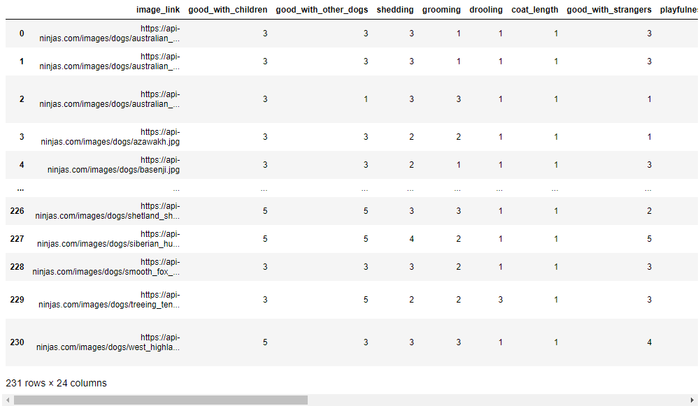
To visualize the data the team used Pandas DataFrame. Shown below is the raw data extracted from the API.
data = pd.DataFrame(ls_dogs)
display(data)
Before we do anything with the dataset, the team first verifies the datatype, missing values, and erroneous data. Shown below are the data types of each column.
display(data.dtypes)
The team verified that all numerical columns are of type int or float from the output. In addition, there are only two object datatypes: image_link and name. These two object datatype was expected, given that those columns are strings. Therefore all data types are correct. The next step is to check if the dataset has missing values. NaN represents missing values.
display(data.isna().sum())
The count of missing values per column is displayed. From this, the team verified that there are no missing values in the dataset. The next step is to check for erroneous data (extreme outliers). This step is done by displaying the range of values for each numerical column.
print("Column value range:\n")
for col_name in data.columns[1:-1]:
    print(f"{col_name} has a value range of {data[col_name].min()} "
          f"to {data[col_name].max()}.")
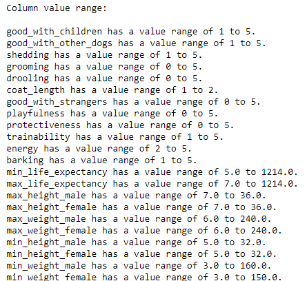
In the output, the team observed that min_life_expectancy and max_life_expectancy have erroneous data, a dog with 1214 expected life years. So the team checked the dog’s name and searched for the correct value.
old = data.loc[data['max_life_expectancy'] >= 1214.0, 'name'].index[0]
print(f"In the database, {data.loc[old, 'name']} has minimum life "
      f"expectancy of {data.loc[old, 'min_life_expectancy']} and "
      f" maximum life expectancy of {data.loc[old, 'max_life_expectancy']}.")
From the website of dogtime.com, Small Munsterlander has a min_life_expectancy of 12 and max_life_expectancy of 14. The error might have been caused by the accidental removal of the hyphen in 12-14 years, resulting in 1214 years. The team corrected this in the dataset. [5]
data.loc[old, 'min_life_expectancy'] = 12
data.loc[old, 'max_life_expectancy'] = 14
The team verified the value range of minimum and maximum life expectancy again.
print("Column value range:\n")
for col_name in ['min_life_expectancy', 'max_life_expectancy']:
    print(f"{col_name} has a value range of {data[col_name].min()} "
          f"to {data[col_name].max()}.")
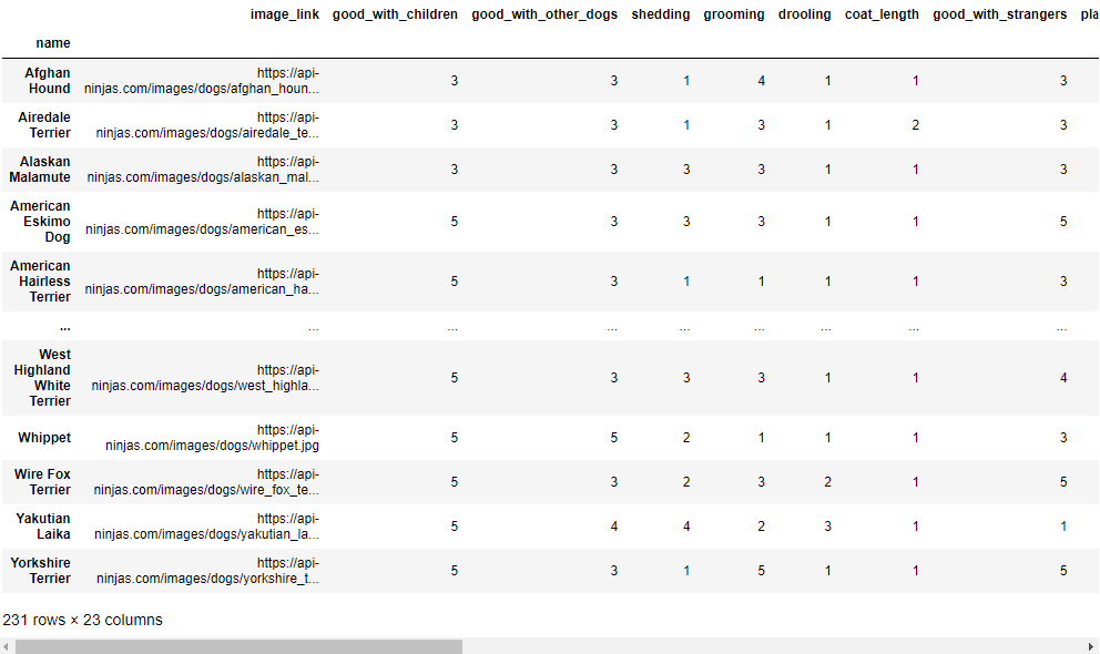
The numerical columns values were now all cleaned and within the reasonable range. The last step in data cleaning is to sort the dataframe based on name and set it as the index. Shown below is the updated database.
data = data.sort_values(by='name').set_index('name')
display(data)
Feature Engineering
Life expectancy, height, and weight were over-represented in the dataset by having more than one column that described them. To address this, the team created a new column to represent the average of their values.
- For life expectancy, the average of the min and max life expectancy was set as a new column called
ave_life_expectancy. - For height and weight, the average of min and max for both sexes will be set as a new column called
ave_heightandave_weight, respectively.
data['ave_life_expectancy'] = (data['min_life_expectancy'] +
                               data['max_life_expectancy']) / 2
data['ave_height'] = (data['max_height_male'] + data['max_height_female'] +
                      data['min_height_male'] + data['min_height_female']) / 4
data['ave_weight'] = (data['max_weight_male'] + data['max_weight_female'] +
                      data['min_weight_male'] + data['min_weight_female']) / 4
These three columns: ave_life_expectancy, ave_height, and ave_weight, represent a measurement that has a scale different from other columns, which has a scale of 1 to 5 (some start at 0). To solve this scaling issue, the team binned these measurements into discrete values of 1 to 5, with 5 being the highest value.
dog_data = data.copy(deep=True)
cols_bin = ['ave_life_expectancy', 'ave_height', 'ave_weight']
labels = [1, 2, 3, 4, 5]

for col in cols_bin:
    boundaries = data[col].value_counts(bins=5, sort=False).index
    bins = []
    for i, boundary in enumerate(boundaries):
        if i == 0:
            bins.append(math.floor(boundary.left))
        else:
            bins.append(round(boundary.left))
        if i == 4:
            bins.append(math.floor(boundary.right))

    dog_data[col] = pd.cut(x=dog_data[col], bins=bins, labels=labels,
                       include_lowest=True)

# Change to int datatype
dog_data = dog_data.astype({'ave_life_expectancy': 'int', 'ave_height': 'int',
                    'ave_weight': 'int'})
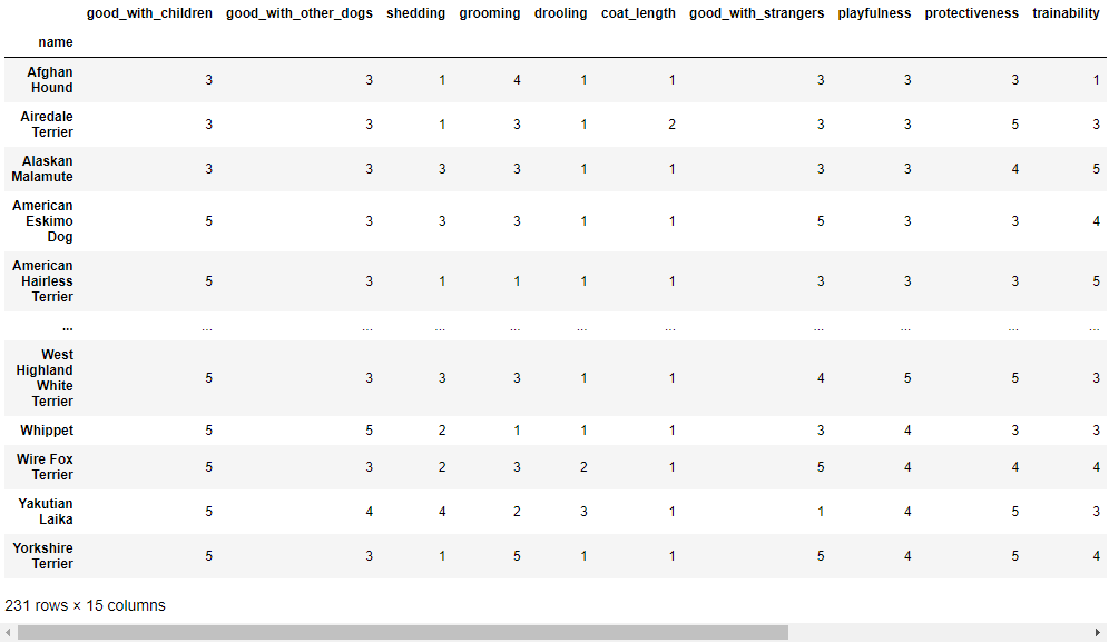
Next step is to drop any unnecessary/redundant columns, retaining only our 15 features as described in the Data Description section above.
# Drop the unnecessary columns
df = dog_data.drop(columns=['image_link', 'min_life_expectancy',
                        'max_life_expectancy', 'max_height_male',
                        'max_height_female', 'min_height_male',
                        'min_height_female', 'max_weight_male',
                        'max_weight_female', 'min_weight_male',
                        'min_weight_female'])
display(df)
# Set up of other necessary variables
# Equivalent numpy of our dataframe.
X = df.to_numpy()

# Array of features
feature_arr = np.array(list(df.columns))

# List of string format features (english equivalent of column names)
feature_str = ['Good with Children', 'Good with Other Dogs', 'Shedding',
               'Grooming', 'Drooling', 'Coat Length', 'Good with Strangers',
               'Playfulness', 'Protectiveness', 'Trainability', 'Energy',
               'Barking', 'Average Life Expectancy', 'Average Height',
               'Average Weight']

# Array of dogs
dog_arr = np.array(list(df.index))

# Figure caption
fig_num = 1
def fig_caption(title, caption):
    """Print figure caption on jupyter notebook"""
    global fig_num
    display(HTML(f"""<p style="font-size:11px;font-style:default;"><b>
                     Figure {fig_num}. {title}.</b><br>{caption}</p>"""))
    fig_num += 1
Exploratory Data Analysis
According to American Kennel Club these 15 features can be grouped together into 4 categories. Shown below are the category of each feature. [2]
- Social
- Playfulness
- Good with Other Dogs
- Good with Stangers
- Good with Children
- Personality
- Energy
- Barking
- Trainability
- Protectiveness
- Physical
- Shedding
- Grooming
- Coat Length
- Drooling
- Size and Life
- Life Expectancy
- Heigth
- Length
The following plots shows the distributions of dogs according to each of those 15 features.
Social
cols_index = [0, 1, 6, 7]
for col in cols_index:
    sub_df = df[feature_arr[col]].value_counts().sort_index()
    fig, ax = plt.subplots(figsize=(8, 5))
    ax.bar(sub_df.index, sub_df.values, color="#DA5F70")
    print('\n\n')
    ax.set_xlabel(f"{feature_str[col]} scale")
    ax.set_ylabel('Dog Count')
    ax.set_title(f'Distribution of Dogs with {feature_str[col]} scale')
    ax.xaxis.set_major_locator(MaxNLocator(integer=True))
    plt.show()
    fig_caption(f'Distribution of Dogs with {feature_str[col]} scale', '')
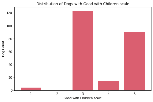
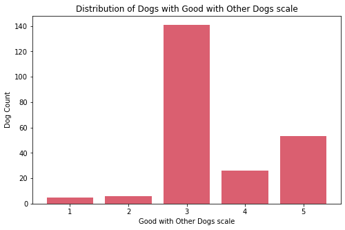
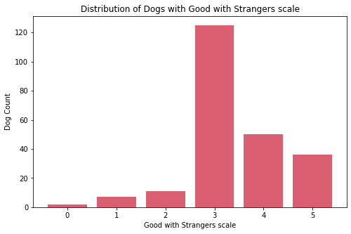
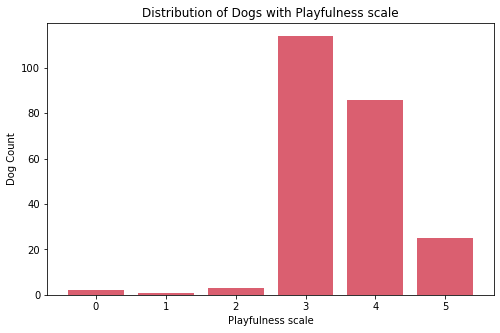
Insights:
- On the four features for social traits, most dogs are classified as middle value.
- There are few dogs that are socially not good with strangers, other dogs, and children.
Personality
cols_index = [8, 9, 10, 11]
for col in cols_index:
    sub_df = df[feature_arr[col]].value_counts().sort_index()
    fig, ax = plt.subplots(figsize=(8, 5))
    ax.bar(sub_df.index, sub_df.values, color="#DA5F70")
    print('\n\n')
    ax.set_xlabel(f"{feature_str[col]} scale")
    ax.set_ylabel('Dog Count')
    ax.set_title(f'Distribution of Dogs with {feature_str[col]} scale')
    ax.xaxis.set_major_locator(MaxNLocator(integer=True))
    plt.show()
    fig_caption(f'Distribution of Dogs with {feature_str[col]} scale', '')
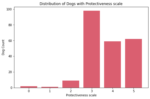
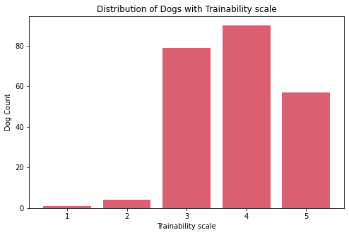
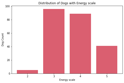
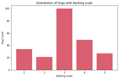
Insights:
- Most dogs have protective nature.
- There are about 57 very trainable dogs.
- Most dogs have middle value of energy. There are five dogs who are the lowest in this scale. Upon further exploration these are:
Basset Hound,Broholmer,Neapolitan Mastiff,Perro de Presa Canario, andPyrenean Mastiff. - Most dogs have middle value of barking with almost balance count on both extremes.
Physical
cols_index = [2, 3, 4, 5]
for col in cols_index:
    sub_df = df[feature_arr[col]].value_counts().sort_index()
    fig, ax = plt.subplots(figsize=(8, 5))
    ax.bar(sub_df.index, sub_df.values, color="#DA5F70")
    print('\n\n')
    ax.set_xlabel(f"{feature_str[col]} scale")
    ax.set_ylabel('Dog Count')
    ax.set_title(f'Distribution of Dogs with {feature_str[col]} scale')
    ax.xaxis.set_major_locator(MaxNLocator(integer=True))
    plt.show()
    fig_caption(f'Distribution of Dogs with {feature_str[col]} scale', '')
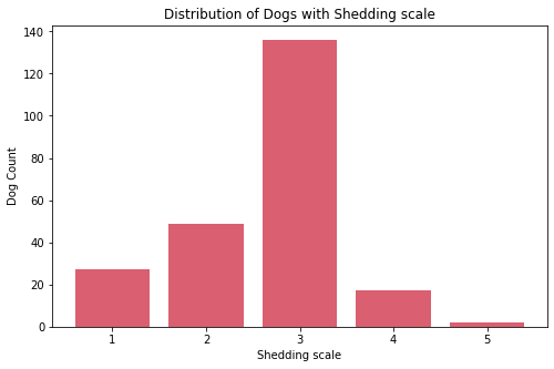
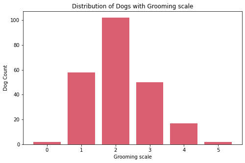
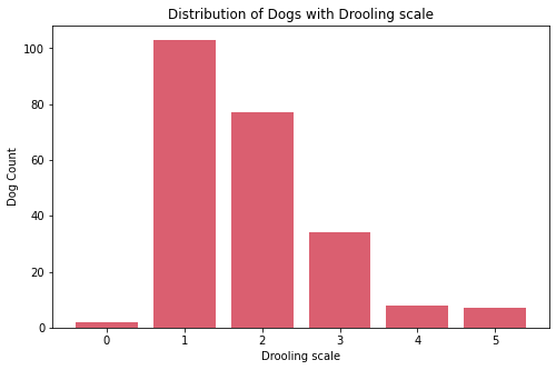
Insights:
- Most dogs have middle value in shedding. Very few have high shedding value these are:
Bernese Mountain Dog, andCzechoslovakian Vlcak. - Most dogs requires less grooming. Very few requires high maintenance in grooming these are:
Bichon Frise, andYorkshire Terrier. - Most dogs drool less. Very few are the dogs that are always drooling, these are:
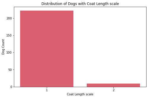
Bloodhound,Dogue de Bordeaux,Neapolitan Mastiff,Newfoundland,Pyrenean Mastiff,Saint Bernard, andSpanish Mastiff. - Almost all dogs have coat length 1. Very few dogs have coat length 2, these are:
Airedale Terrier,Barbet,Black Russian Terrier,Brussels Griffon,Chihuahua,Chinese Crested,Collie,Dachshund, andEnglish Cocker Spaniel.
Size and Life
cols_index = [12, 13, 14]
for col in cols_index:
    sub_df = df[feature_arr[col]].value_counts().sort_index()
    fig, ax = plt.subplots(figsize=(8, 5))
    ax.bar(sub_df.index, sub_df.values, color="#DA5F70")
    print('\n\n')
    ax.set_xlabel(f"{feature_str[col]} scale")
    ax.set_ylabel('Dog Count')
    ax.set_title(f'Distribution of Dogs with {feature_str[col]} scale')
    ax.xaxis.set_major_locator(MaxNLocator(integer=True))
    plt.show()
    fig_caption(f'Distribution of Dogs with {feature_str[col]} scale', '')
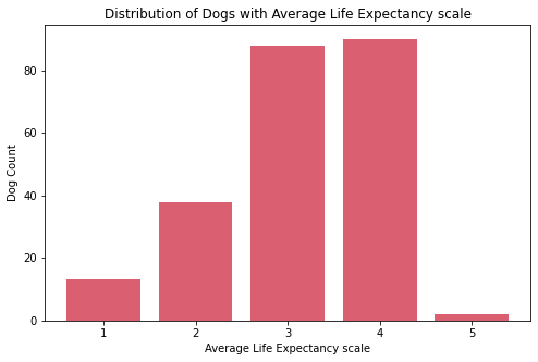

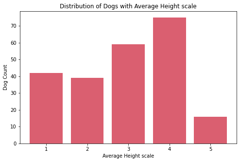
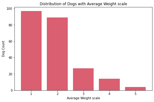
Insights:
- The
ave_life_expectancyscale of dogs are mostly on 3 and 4. - The most common
ave_heightscale of dogs is 4 while the least common is 5. There are only few breeds of dogs which are the tallest on the theave_heightscale. - The
ave_weightscale of dogs are mostly on 1 and 2. There are only few breeds of dogs which are the heaviest on the theave_weightscale.
Features Correlation Heatmap
corr = df.corr()
mask = np.triu(np.ones_like(corr))
fig, ax = plt.subplots(figsize=(18, 9))
ax = sns.heatmap(corr, annot=True, center=0, cmap='coolwarm_r', mask=mask,
                 yticklabels=feature_str, xticklabels=feature_str)
ax.tick_params(axis='y')
ax.tick_params(axis='x', labelrotation=45)
plt.show()
fig_caption(f'Correlation Heatmap of Features', '')
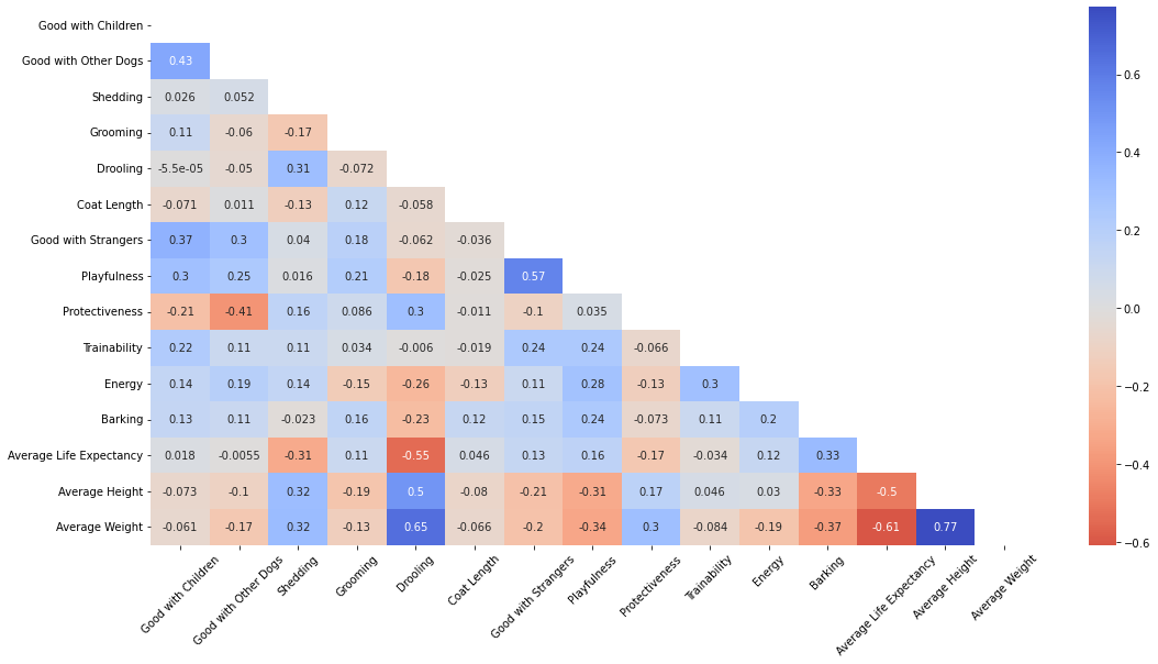
Insights:
- Average height strongly correlated with average weight. These are eminent on breeds such as Neapolitan Mastiff, Newfoundland, and Pyrenean Mastiff.
- Dogs that are playful are generally also good with strangers. Dogs that are good with other dogs are good with kids as well.
- Some features are negatively correlated such as protectiveness and good with other dogs, as protective dogs that guard their owners well are not receptive with other dogs.
- Heavy dogs tend to have lower life expectancies as well. One reason for this is that larger dogs die earlier because they age significantly faster compared to smaller dogs.
Height and Weight Relationship Plot
The team looked into the specific relationship of height and weight.
# Height vs Weight (Positive Correlation)
fig, ax = plt.subplots(figsize=(12, 6))
ax = sns.regplot(x=data['ave_weight'], y=data['ave_height'], color="#DA5F70")
ax.set_title('Height vs Weight Scatter Diagram')
ax.set_xlabel('Average Weight')
ax.set_ylabel('Average Height')
plt.show()
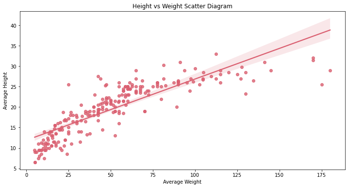
Insight:
- There is a linear relationship between the variables ( Average weight against average height)
- It can be seen that some dogs have heaver weight but have the same height with dogs with lighter weight, since we are only getting the height of dogs and didn’t include their width/length.
Results and Discussion
Dimensionality Reduction
Principal Component Analysis (PCA)
The team used Principal Component Analysis or PCA to determine the top features that defines most of the variance. sklearn PCA method was used.
# PCA
pca = PCA()
X_center = (X - X.mean(axis=0)) / X.std(axis=0)
pca.fit_transform(X_center)
var_exp = pca.explained_variance_ratio_
w = pca.components_
X_new = np.dot(X_center, w)
The team determined the minimum value of principal components (PCs) to achieved 80% cumulative variance explained. Shown below are the plot for the variance explained ratio and its cumulative.
# Plot of variance explained and Cummulative Variance Explained
fig, ax = plt.subplots(figsize=(8, 5))
ax.plot(range(1, len(var_exp)+1), var_exp.cumsum(), 'o-', label='cumulative')
ax.plot(range(1, len(var_exp)+1), var_exp, 'o-', label='individual')

ax.set_ylim(0, 1.05)
ax.axhline(0.8, ls='--', color='#DA5F70')
ax.axvline(8, ls='--', color='#DA5F70')
ax.set_xlabel('Principal Component')
ax.set_ylabel('Variance Explained')
ax.set_title('Variance Explained and Cumulative Variance Explained of PCs')
ax.legend()
plt.show()
fig_caption('Variance Explained and Cumulative Variance Explained of PCs', '')
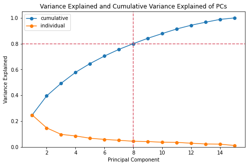
min_pcs = np.argmax(var_exp.cumsum() >= 0.80) + 1
print(f"The minimum PCs to achieve at least 80% cummulative variance explained is "
      f"{min_pcs}.")
The team plotted the transformed original features onto the first two PCs.
# Plot the transformed data on the first 2 PCs w/ transformed features
fig, ax = plt.subplots(1, 1, subplot_kw=dict(aspect='equal'), figsize=(10, 10))
ax.scatter(X_new[:,0], X_new[:,1])
for feature, vec in zip(feature_arr, w):
    ax.arrow(0, 0, 5*vec[0], 5*vec[1], width=0.02, ec='none', fc='r')
    ax.text(5.5*vec[0], 5.5*vec[1], feature, ha='center', color='r', size=10)
ax.set_xlabel('PC1', size=15)
ax.set_ylabel('PC2', size=15)
ax.set_title('Dogs Dataset on PC1 and PC2 axis', size=20)
plt.show()
fig_caption('Dogs Dataset on PC1 and PC2 axis', '')
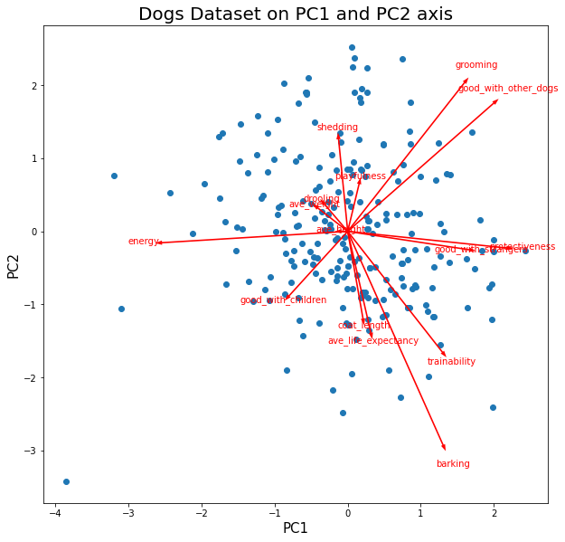
Insights:
Coordinates
- Positive PC1 is mainly described by high values of features:
good_with_other_dogs,good_with_strangers,barking. - Negative PC1 is mainy described by high values of features:
energy, andprotectiveness. - Negative PC2 is mainly described by high values of features:
barking,trainability. - Positive PC2 is mainly described by high values of features:
grooming,good_with_other_dogs.
Correlations
protectiveness, andenergyare fairly correlated. These features are anticorrelated togood_with_strangers.groomingandgood_with_other_dogsare fairly correlated.barkingandtrainabilityare fairly correlated.groomingandgood_with_other_dogsis fairly orthogonal totrainabilityandbarking. This suggest independence between those features.
Clusters
- There are no observable clustering in the data points.
Funnels
- There are no observable funneling in the data points.
Voids
- There are no observable voids in the data points. This suggests that all combination of features are possible.
The following plots shows the feature contributing to the first 8 PCs.
for i in range(min_pcs):
    fig, ax = plt.subplots()
    order = np.argsort(np.abs(w[:, i]))[-5:]
    ax.barh([feature_arr[o] for o in order], w[order, i])
    ax.set_title(f'PC{i+1}')
    ax.set_xlabel('Feature Factor')
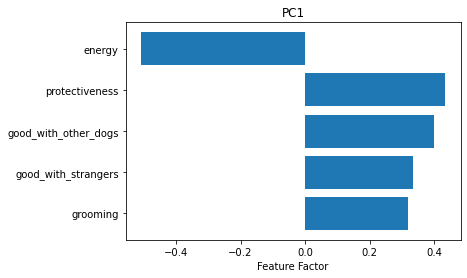
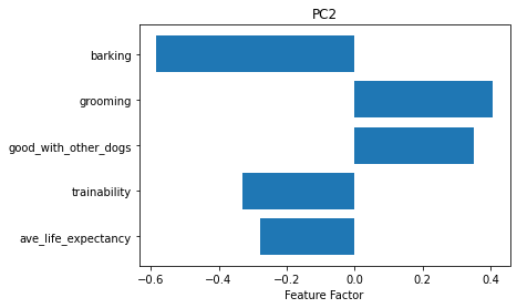
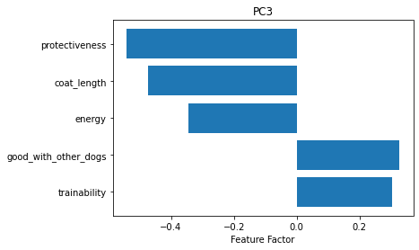
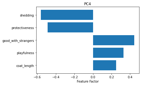
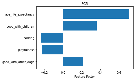
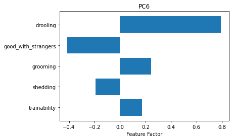
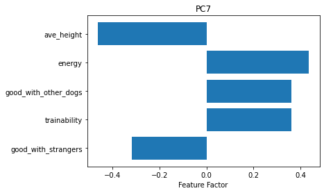
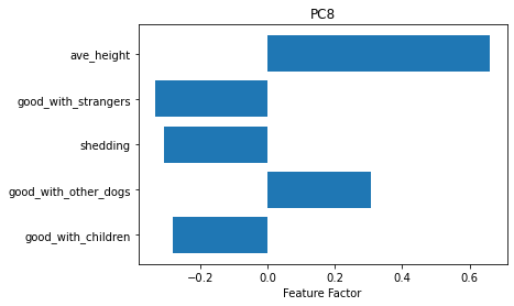
Insights:
- PC1 - Negative PC1 corresponds to
energyandprotectivenesswhile positive PC1 corresponds togood_with_other_dogsandbarking. - PC2 - Negative PC2 corresponds to
barkingandtrainabilitywhile positive PC2 corresponds togrooming, andgood_with_other_dogs. - PC3 - Negative PC3 corresponds to
coat_lengthandenergywhile positive PC3 corresponds toprotectiveness, andgood_with_other_dogs. - PC4 - Negative PC4 corresponds to
sheddingwhile positive PC4 corresponds toprotectiveness, andgood_with_strangers. - PC5 - Negative PC5 corresponds to
playfulnessandsheddingwhile positive PC5 corresponds toave_life_expectancy, andgood_with_children. - PC6 - Negative PC6 corresponds to
good_with_strangersandsheddingwhile positive PC6 corresponds todrooling, andgrooming. - PC7 - Negative PC7 corresponds to
ave_heightandgood_with_strangerswhile positive PC7 corresponds totrainability, andenergy. - PC8 - Negative PC8 corresponds to
good_with_strangersandgood_with_childrenwhile positive PC8 corresponds toave_height, andgood_with_other_dogs.
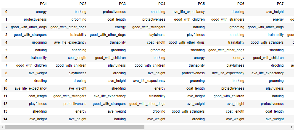
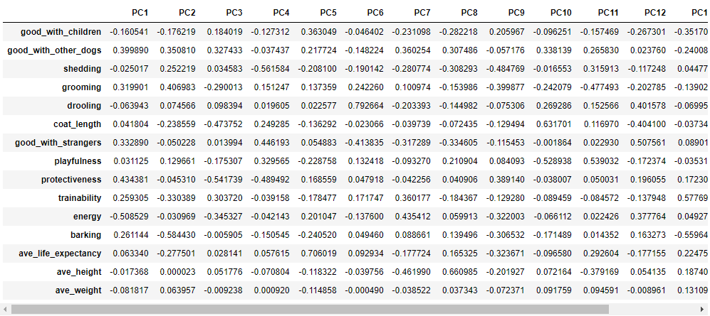
Shown below are the top influencing features per PCs.
pc_dict = {}
for i in range(len(w)):
    pc_dict.update({f"PC{i+1}": feature_arr[(np.argsort(-np.abs(w[:, i])))]})
pc_features = pd.DataFrame(pc_dict)
display(pc_features)
Here are the exact values:
pc_dict = {}
for i in range(len(w)):
    pc_dict.update({f"PC{i+1}": w[:, i]})
pc_values = pd.DataFrame(pc_dict, index=feature_arr)
display(pc_values)
Using the first 8 PCs, the top features were determined to create to reduced-dimension dataframe.
imp_feature = []
for col_i in range(min_pcs):
    for row_i in range(len(pc_features)):
        if pc_features.iloc[row_i, col_i] not in imp_feature:
            imp_feature.append(pc_features.iloc[row_i, col_i])
            break
print(f"The reduced-dimension has {len(imp_feature)} important features.")
Insights:
- The team looked at the top features per principal component and they are energy, barking, protectiveness, shedding, average life expectancy, drooling, average height, and good with strangers, respectively.
- For PC1, this principal component increases as energy decreases, while for PC2, the PC increases as barking decreases.
- PC3 increases as protectiveness decreases, PC4 increases as shedding decreases, PC5 increases as average life expectancy increases, and PC6 increases as drooling decreases.
- PC7 increases as average height decreases and while energy increases, and lastly PC8 increases as average height increases and good with strangers decreases.
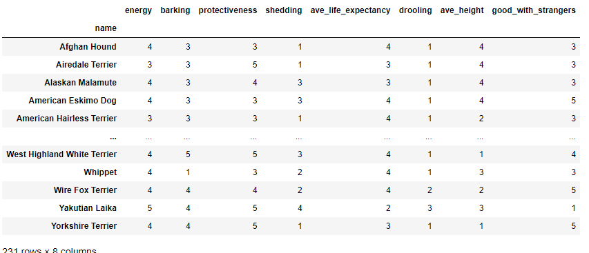
The reduced feature dataframe is shown below.
# Get the reduced dataset
df_red = df.copy(deep=True)[imp_feature]
X_red = df_red.to_numpy()
display(df_red)
Non-negative Matrix-Factorization (NMF)
The team used Non-negative matrix-factorization (NMF) to determine the features cluster and dog clusters. First in order to determine the number of latent factor, the team used Frobenius norm of the original matrix vs the reconstructed matrix at different values of latent factors (k). Shown below is the plot of Frobenius norm at k value from 2 to 15.
f_norm = []
for k in range(2, len(feature_arr) + 1):
    nmf = NMF(n_components=k, max_iter=10_000)
    U = nmf.fit_transform(X)
    V = nmf.components_.T
    f_norm.append(((X - U @ V.T) ** 2).sum())

# Plot Frobenius norm
fig, ax = plt.subplots()
ax.plot(range(2, len(f_norm) + 2), f_norm, 'o-')
ax.set_xlabel('k')
ax.set_ylabel('Frobenius norm')
ax.set_title('Frobenius norm vs Latent Factors (k)')
plt.show()
fig_caption('Frobenius norm vs Latent Factors (k)', '')
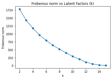
The “knee” of the plot is not clearly defined. So, the team proceed to analyze the numerical value of frobenius norm to determine at whch value of k that the reduction of reconstruction error has diminishing returns.
# Analyzing the number
f_diff = np.array([f_norm[i-1] - f_norm[i]
                   for i in range(1, len(f_norm))])
min_lfs = np.where(f_diff < 150)[0][0] + 3  # f_diff starts at LF 3
print(f"The optimal number of latent factors is {min_lfs}.")
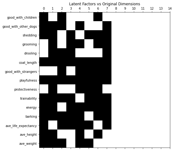
Shown below is the plot of latent factors vs Original Dimensions, where white box corresponds to the zero (0) factor.
nmf = NMF(n_components=min_lfs, max_iter=1_000)
U = nmf.fit_transform(df)
V = nmf.components_.T

fig, ax = plt.subplots(figsize=(8, 8))
ax.spy(V)
ax.set_xticks(range(len(feature_arr)))
ax.set_yticks(range(len(feature_arr)))
ax.set_yticklabels(feature_arr)
ax.set_title('Latent Factors vs Original Dimensions')
plt.show()
fig_caption('Latent Factors vs Original Dimensions', '')
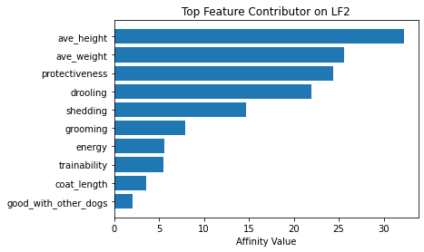
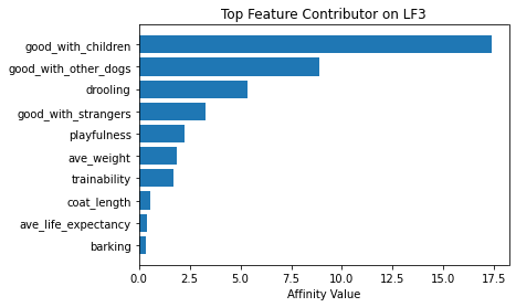
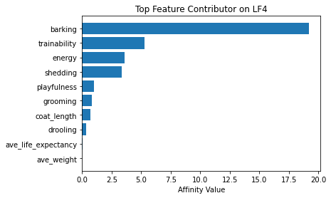
Now using seven latent factors, the team determined the defining characteristics and labeled each clusters.
# Plot of feature influence on Latent Factors
for i in range(min_lfs):
    fig, ax = plt.subplots()
    order = np.argsort(np.abs(V[:, i]))[-10:]
    ax.barh([feature_arr[o] for o in order], V[order, i])
    ax.set_title(f'Top Feature Contributor on LF{i+1}')
    ax.set_xlabel('Affinity Value')
plt.show()
fig_caption('Top Feature Contributor of LF1 to LF8', '')
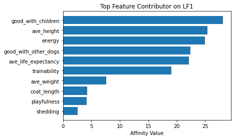
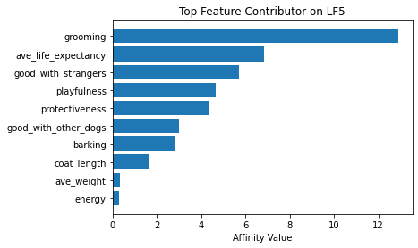
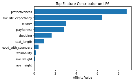
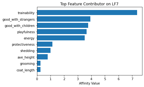
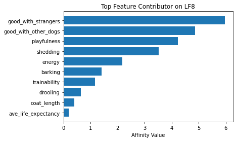
Insights:
- Latent Factor 1 - Energetic Big Child-friendly Dogs
- Latent Factor 2 - Big Protective Dogs
- Latent Factor 3 - High Maintenance Socially Well Dogs
- Latent Factor 4 - Loud Dogs
- Latent Factor 5 - Energetic Tall Dogs
- Latent Factor 6 - Protective yet Playful Dogs
- Latent Factor 7 - Easily Trained ActiveDogs
- Latent Factor 8 - Socially Behaved Dogs
lf_labels = ['Energetic Big Child-friendly Dogs', 'Big Protective Dogs',
             'High Maintenance Socially Well Dogs',
             'Very Vocal Dogs', 'Energetic Tall Dogs',
             'Protective yet Playful Dogs', 'Easily Trained ActiveDogs',
             'Socially Behaved Dogs']
Using these latent factors labels, the affinity of each dog to a cluster was determined. Shown below is the translated value into first 2 PCs with color representing unique cluster
# Clustering by assigning them to the latent factor with the highest weight
fig, ax = plt.subplots(figsize=(8, 6))
pca_nmf = PCA(2)
ax.scatter(*pca_nmf.fit_transform(X_center).T,
           c=U.argmax(axis=1), cmap='Set1')
ax.set_xlabel('PC1')
ax.set_ylabel('PC2')
ax.set_title('PC Axis with Clustering')
plt.show()
fig_caption('PC Axis with Clustering', '')
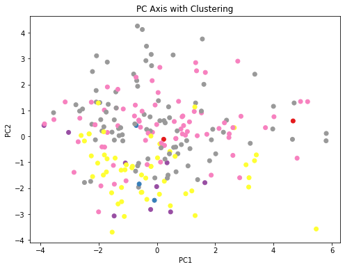
The clusters of each dog was determined. Some cluster doesn’t have any member this is because dogs that might be classified into these clusters have more affinity towards other clusters.
# Clustering
df_cluster = df.copy()
df_cluster['nmf_cluster'] = U.argmax(axis=1)

for i in range(8):
    nmf_cluster = list(df_cluster[df_cluster['nmf_cluster'] == i].index)
    print(f"{lf_labels[i]}:\n {nmf_cluster}\n")
Information Retrieval (IR)
To determine the performance of dimensionality reduction the team perform information retrieval on both datasets that are full 15 features and reduced to 8 features. The similarity score used for information retrival is cosine distance because all of the data in our dataset are non-negative.
def nearest_dog(query, obj, dog_arr, k):
    """Returns the top k nearest dog to the query from the obj."""
    near_k = np.argsort([distance.cosine(query, vec) for vec in obj])[:k]
    near_dog = dog_arr[near_k]
    return near_dog

top_count = 10
dog_index = 167
print(f"IR will retrieved the top {top_count} nearest dog from the query. The "
      f"sample dog querry is {dog_arr[dog_index]}.")
Instead of asking for the 15 features to come up with a recommended dog, the team reduced it to 8 questions (features). This reduced questions still yields a significant % accuracy base from the original dimensions results.
# Sample original dimension query
sample_orig = X[dog_index, :]

# Get the top 20% nearest from the query
search_orig = nearest_dog(sample_orig, X, dog_arr, top_count)
print(f"The top {top_count} nearest dog from our query "
      f"are:\n\n{search_orig}\n\n")

# Sample reduced-dimension query
sample_red = X_red[dog_index, :]

# Get the top 20% nearest from the query
search_red = nearest_dog(sample_red, X_red, dog_arr, top_count)
print(f"Using the reduced features, the top {top_count} nearest dog from "
     f"our query are:\n\n{search_red}\n\n")

# Get the % match between the original and reduced-dimension
count = 0
for i in search_orig:
    if i in search_red:
        count += 1
pct_match = count / top_count * 100
print(f"The percent match between the original search and reduced-dimension "
      f"search is {pct_match:.0f}%")
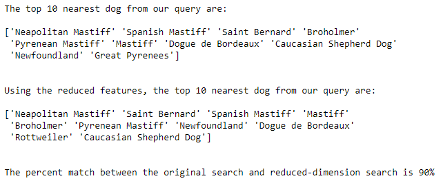
This high percentage match indicates that instead of asking for all 15 features the program could focus only on the 8 important features.
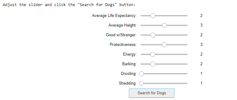
Which Dog Should I Select?
Going back to the question “Which Dog Should I Select”, the team develop an interactive jupyter notebook widget. This interface will return the top 3 recommended dogs base on the user input.
def search_query():
user_query = np.array([energy.value, barking.value, protectiveness.value,
shedding.value, ave_life_expectancy.value,
drooling.value, ave_height.value,
good_with_strangers.value])
# Search the top 3 dogs
search_results = nearest_dog(user_query, X_red, dog_arr, 3)
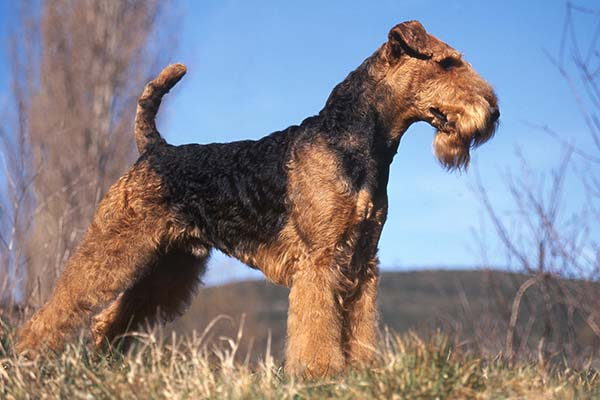
# Display the dog image
for dog_name in search_results:
resp = requests.get(data.loc[dog_name, 'image_link'])
img = Image.open(BytesIO(resp.content))
print(dog_name)
display(img)
# Input set up
# style = {'description_width': 'initial'}
style = {'description_width': '150px'}
layout = {'width': '400px'}
ave_life_expectancy = widgets.IntSlider(
min=1, max=5,step=1, description='Average Life Expectancy:',
style=style, layout=layout)
ave_height = widgets.IntSlider(
min=1, max=5,step=1, description='Average Height:',
style=style, layout=layout)
good_with_strangers = widgets.IntSlider(
min=1, max=5,step=1, description='Good w/Stranger:',
style=style, layout=layout)
protectiveness = widgets.IntSlider(
min=1, max=5,step=1, description='Protectiveness:',
style=style, layout=layout)
energy = widgets.IntSlider(
min=1, max=5,step=1, description='Energy:',
style=style, layout=layout)
barking = widgets.IntSlider(
min=1, max=5,step=1, description='Barking:',
style=style, layout=layout)
drooling = widgets.IntSlider(
min=1, max=5,step=1, description='Drooling:',
style=style, layout=layout)
shedding = widgets.IntSlider(
min=1, max=5,step=1, description='Shedding:',
style=style, layout=layout)
# Button and Output
butt = widgets.Button(description='Search for Dogs')
outt = widgets.Output()
layout = widgets.Layout(align_items='center')
def on_butt_clicked(b):
with outt:
clear_output()
search_query()
butt.on_click(on_butt_clicked)
# Display Interactive Widgets
print('Adjust the slider and click the "Search for Dogs" button:')
widgets.VBox([ave_life_expectancy, ave_height, good_with_strangers,
protectiveness, energy, barking, drooling, shedding,
butt, outt], layout=layout)
Conclusion
The team looked at 231 different breeds of dogs and found that there are features that contribute the most in selecting the preferred dogs. These features are namely energy, barking, protectiveness, shedding, average life expectancy, drooling, average height, and good with strangers. There are features that correlate positively with other features - for example, dogs that are playful are generally also good with strangers. Dogs that are good with other dogs are good with kids as well. Heavy dogs tend to have lower life expectancies as well.
Using the top features that emerged from doing the Principal Components Analysis, the team did Information Retrieval, looked at the top 10 results, and compared it with the Information Retrieval using all the features. Interestingly, 90% of the results matched. We can now answer the question “Which dog should I select?” by asking the features that contribute the most in selecting the right dog breed.
So if you ever find yourself paw-sing and reflecting on getting a furry friend, give our team a call. We’re the right tree to bark up. We’re excited to be part of your journey in selecting the paw-fect dog for you.
Recommendations
The system may be further improved by conducting the following:
- Other clustering methods may be explored outside of NMF. K-means clustering or Density based clustering methods such as DBSCAN or OPTICS may be considered in grouping the different breeds of dogs before doing the information retrieval. With this, the system can determine the preferred characteristics of the person and then look at the dogs within specific clusters, not necessarily looking into the whole dataset every query.
- Aside from only looking at the top features per principal component, future studies may consider on taking into account ‘obvious’ values on select features. For example, the most preferred average life expectancy is 5, since people generally want their dogs to live the longest.
- Adding other relevant features such as price and availability in the region or country may also be considered.
References
[1] api-ninjas.com (n.d.) Build Real Projects with Real Data. Retrieved November 25, 2022 at https://api-ninjas.com/api/dogs
[2] yahoo.com (2020, July 22) Here’s Why Your Dog Knows When It’s Time For Food and Walks, According to Experts. Retrieved December 1, 2022 at https://www.yahoo.com/lifestyle/am-imagining-things-dog-tell-200136032.html
[3] bing.com (n.d.) What breed is that dog?. Retrieved December 6, 2022 at https://www.bing.com/visualsearch/Microsoft/WhatDog
[4] American Knnel Club (n.d.) Dog Breeds. Retrieved December 6, 2022, from https://www.akc.org/dog-breeds/
[5] dogtime.com (n.d.) Small Munsterlander Pointer. Retrieved November 30, 2022 at https://dogtime.com/dog-breeds/small-munsterlander-pointer#/slide/1.
ACKNOWLEDGEMENT
I completed this project with my Learning Team, which consisted of Ma. Lair Balogal, Felipe Garcia Jr., Vanessa delos Santos, and Josemaria Likha Umali.