
Dota 2 Match Analysis: Unleashing the Potential of LightGBM Machine Learning Techniques
Published:

EXECUTIVE SUMMARY
Dota 2, a leading multiplayer online battle arena (MOBA) game, engages two teams of five players in a strategic contest to destroy their opponent’s “Ancient” structure while safeguarding their own. With its prominent presence in the esports domain, insights into the determinants of match outcomes hold significant value.
In each match, Radiant and Dire teams consist of five players who adopt specialized roles based on their chosen heroes. The game map comprises diverse elements, including team bases, lanes, shops, and Roshan’s lair. Players focus on hero upgrades, item acquisitions, and enemy base destruction to achieve victory.
This study employs machine learning algorithms to analyze collected data, establish baseline scores, and optimize model performance, yielding high-accuracy models for predicting Dota 2 match outcomes. Nevertheless, the reduction of the dataset due to time constraints and computational resources presents a limitation to the study’s scope.
Future research can investigate additional models and optimization approaches to augment or supplement existing findings, further advancing our understanding and predictive capabilities for Dota 2 match outcomes.
HIGHLIGTHS
- Showcased the application of Bayesian Optimization and its impact on enhancing accuracy levels.
- Illustrated the implementation of Light Gradient Boosting alongside hyperparameter tuning.
- Explored the utilization of various Classification Models for diverse predictions.
- Identified gold as the most influential predictor in determining match outcomes.
- Emphasized the importance of Feature Engineering in optimizing model performance and efficiency.
METHODOLOGY
The overarching methodology of this project focuses on employing various machine learning models, particularly LightGBM, to accurately predict Dota 2 match outcomes. The following steps outline the process:
- Data Retrieval: Acquiring the relevant dataset for analysis.
- Data Cleaning: Ensuring data quality by removing inconsistencies and inaccuracies.
- Exploratory Data Analysis: Investigating data patterns, relationships, and trends to gain insights.
- Data Preprocessing: Transforming and preparing the data for machine learning models.
- ML Models Simulation: Implementing and comparing the performance of various machine learning models.
- Hyperparameter Optimization: Fine-tuning model parameters to enhance predictive accuracy and efficiency.
Import Libraries
# Data manipulation and analysis
import pandas as pd
import numpy as np

# Data visualization
import seaborn as sns
import matplotlib.pyplot as plt

# Machine learning models and algorithms
from sklearn.neighbors import KNeighborsClassifier
from sklearn.linear_model import Ridge, Lasso, LogisticRegression
from sklearn.tree import DecisionTreeClassifier
from sklearn.svm import LinearSVC, SVC, SVR
from sklearn.ensemble import (RandomForestClassifier,
                              GradientBoostingClassifier,
                              AdaBoostClassifier,
                              ExtraTreesClassifier,
                              VotingClassifier)
from sklearn.neural_network import MLPClassifier
from xgboost import XGBClassifier
from lightgbm import LGBMClassifier
from catboost import CatBoostClassifier

# Machine learning tools and utilities
from mltools import *
from bayes_opt import BayesianOptimization

# Data preprocessing and preparation
from sklearn.preprocessing import StandardScaler

# Ignore warnings
import warnings
warnings.filterwarnings("ignore")
Data Retrieval
The data used in this project is sourced from a Kaggle dataset [5]. The OpenDota API, which could have been an alternative, is no longer a viable option due to its restrictions on non-premium subscribers and the removal of free access to the API.
Data Loading
# loading data
train_data = pd.read_csv('./train_features.csv', index_col='match_id_hash')
test_data = pd.read_csv('./test_features.csv', index_col='match_id_hash')
train_y = pd.read_csv('./train_targets.csv', index_col='match_id_hash')
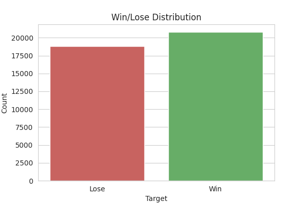
colors = ['#d9534f', '#5cb85c']
# Compute the target value counts
target_counts = train_y['radiant_win'].value_counts()
# Create a plot using seaborn
plt.figure(figsize=(6, 4))
sns.set_style('whitegrid')
ax = sns.barplot(x=target_counts.index,
y=target_counts.values, palette=colors)
ax.set_title('Win/Lose Distribution')
ax.set_xlabel('Target')
ax.set_ylabel('Count')
ax.set_xticklabels(['Lose', 'Win'])
# Save the plot as a PNG file
plt.savefig("images/balance.png")
# Create an HTML img tag to display the image
img_tag = (f'<img src="images/balance.png" alt="balance"'
f'style="display:block; margin-left:auto;'
f'margin-right:auto; width:80%;">')
# display the HTML <img> tag
display(HTML(img_tag))
plt.close()
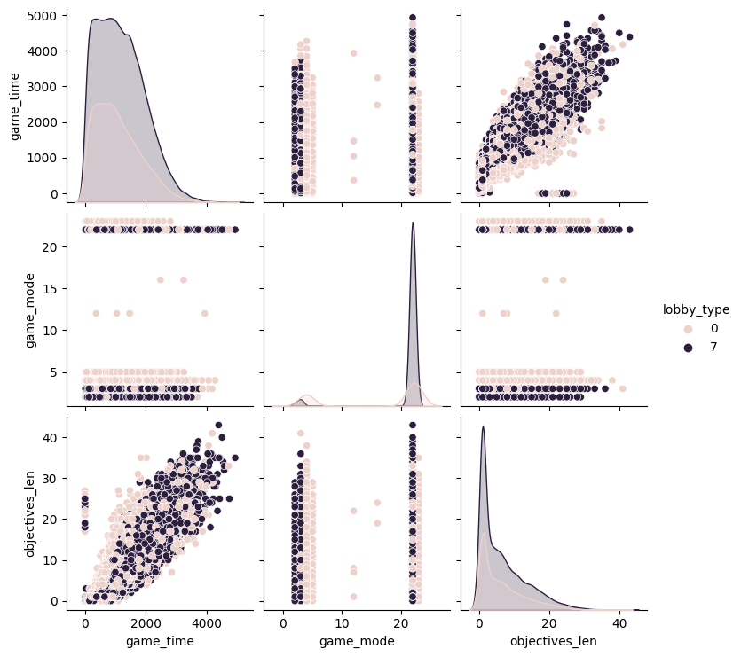
sns.pairplot(train_data.iloc[:,:4], hue='lobby_type')
Data Description
num_rows = train_data.shape[0]
num_cols = train_data.shape[1]
html_table = train_data.head().to_html()
html_table_with_info = f"{html_table} \n <p>Number of Rows: {num_rows}<br>Number of Columns: {num_cols}</p>"

# Print the HTML table
print(html_table_with_info)
| game_time | game_mode | lobby_type | objectives_len | chat_len | r1_hero_id | r1_kills | r1_deaths | r1_assists | r1_denies | r1_gold | r1_lh | r1_xp | r1_health | r1_max_health | r1_max_mana | r1_level | r1_x | r1_y | r1_stuns | r1_creeps_stacked | r1_camps_stacked | r1_rune_pickups | r1_firstblood_claimed | r1_teamfight_participation | r1_towers_killed | r1_roshans_killed | r1_obs_placed | r1_sen_placed | r2_hero_id | r2_kills | r2_deaths | r2_assists | r2_denies | r2_gold | r2_lh | r2_xp | r2_health | r2_max_health | r2_max_mana | r2_level | r2_x | r2_y | r2_stuns | r2_creeps_stacked | r2_camps_stacked | r2_rune_pickups | r2_firstblood_claimed | r2_teamfight_participation | r2_towers_killed | r2_roshans_killed | r2_obs_placed | r2_sen_placed | r3_hero_id | r3_kills | r3_deaths | r3_assists | r3_denies | r3_gold | r3_lh | r3_xp | r3_health | r3_max_health | r3_max_mana | r3_level | r3_x | r3_y | r3_stuns | r3_creeps_stacked | r3_camps_stacked | r3_rune_pickups | r3_firstblood_claimed | r3_teamfight_participation | r3_towers_killed | r3_roshans_killed | r3_obs_placed | r3_sen_placed | r4_hero_id | r4_kills | r4_deaths | r4_assists | r4_denies | r4_gold | r4_lh | r4_xp | r4_health | r4_max_health | r4_max_mana | r4_level | r4_x | r4_y | r4_stuns | r4_creeps_stacked | r4_camps_stacked | r4_rune_pickups | r4_firstblood_claimed | r4_teamfight_participation | r4_towers_killed | r4_roshans_killed | r4_obs_placed | r4_sen_placed | r5_hero_id | r5_kills | r5_deaths | r5_assists | r5_denies | r5_gold | r5_lh | r5_xp | r5_health | r5_max_health | r5_max_mana | r5_level | r5_x | r5_y | r5_stuns | r5_creeps_stacked | r5_camps_stacked | r5_rune_pickups | r5_firstblood_claimed | r5_teamfight_participation | r5_towers_killed | r5_roshans_killed | r5_obs_placed | r5_sen_placed | d1_hero_id | d1_kills | d1_deaths | d1_assists | d1_denies | d1_gold | d1_lh | d1_xp | d1_health | d1_max_health | d1_max_mana | d1_level | d1_x | d1_y | d1_stuns | d1_creeps_stacked | d1_camps_stacked | d1_rune_pickups | d1_firstblood_claimed | d1_teamfight_participation | d1_towers_killed | d1_roshans_killed | d1_obs_placed | d1_sen_placed | d2_hero_id | d2_kills | d2_deaths | d2_assists | d2_denies | d2_gold | d2_lh | d2_xp | d2_health | d2_max_health | d2_max_mana | d2_level | d2_x | d2_y | d2_stuns | d2_creeps_stacked | d2_camps_stacked | d2_rune_pickups | d2_firstblood_claimed | d2_teamfight_participation | d2_towers_killed | d2_roshans_killed | d2_obs_placed | d2_sen_placed | d3_hero_id | d3_kills | d3_deaths | d3_assists | d3_denies | d3_gold | d3_lh | d3_xp | d3_health | d3_max_health | d3_max_mana | d3_level | d3_x | d3_y | d3_stuns | d3_creeps_stacked | d3_camps_stacked | d3_rune_pickups | d3_firstblood_claimed | d3_teamfight_participation | d3_towers_killed | d3_roshans_killed | d3_obs_placed | d3_sen_placed | d4_hero_id | d4_kills | d4_deaths | d4_assists | d4_denies | d4_gold | d4_lh | d4_xp | d4_health | d4_max_health | d4_max_mana | d4_level | d4_x | d4_y | d4_stuns | d4_creeps_stacked | d4_camps_stacked | d4_rune_pickups | d4_firstblood_claimed | d4_teamfight_participation | d4_towers_killed | d4_roshans_killed | d4_obs_placed | d4_sen_placed | d5_hero_id | d5_kills | d5_deaths | d5_assists | d5_denies | d5_gold | d5_lh | d5_xp | d5_health | d5_max_health | d5_max_mana | d5_level | d5_x | d5_y | d5_stuns | d5_creeps_stacked | d5_camps_stacked | d5_rune_pickups | d5_firstblood_claimed | d5_teamfight_participation | d5_towers_killed | d5_roshans_killed | d5_obs_placed | d5_sen_placed | |
|---|---|---|---|---|---|---|---|---|---|---|---|---|---|---|---|---|---|---|---|---|---|---|---|---|---|---|---|---|---|---|---|---|---|---|---|---|---|---|---|---|---|---|---|---|---|---|---|---|---|---|---|---|---|---|---|---|---|---|---|---|---|---|---|---|---|---|---|---|---|---|---|---|---|---|---|---|---|---|---|---|---|---|---|---|---|---|---|---|---|---|---|---|---|---|---|---|---|---|---|---|---|---|---|---|---|---|---|---|---|---|---|---|---|---|---|---|---|---|---|---|---|---|---|---|---|---|---|---|---|---|---|---|---|---|---|---|---|---|---|---|---|---|---|---|---|---|---|---|---|---|---|---|---|---|---|---|---|---|---|---|---|---|---|---|---|---|---|---|---|---|---|---|---|---|---|---|---|---|---|---|---|---|---|---|---|---|---|---|---|---|---|---|---|---|---|---|---|---|---|---|---|---|---|---|---|---|---|---|---|---|---|---|---|---|---|---|---|---|---|---|---|---|---|---|---|---|---|---|---|---|---|---|---|---|---|---|---|---|---|---|---|---|---|---|---|
| match_id_hash | |||||||||||||||||||||||||||||||||||||||||||||||||||||||||||||||||||||||||||||||||||||||||||||||||||||||||||||||||||||||||||||||||||||||||||||||||||||||||||||||||||||||||||||||||||||||||||||||||||||||||||||||||||||||||||||||||||||||||||||||||||||
| a400b8f29dece5f4d266f49f1ae2e98a | 155 | 22 | 7 | 1 | 11 | 11 | 0 | 0 | 0 | 0 | 543 | 7 | 533 | 358 | 600 | 350.93784 | 2 | 116 | 122 | 0.000000 | 0 | 0 | 1 | 0 | 0.000000 | 0 | 0 | 0 | 0 | 78 | 0 | 0 | 0 | 3 | 399 | 4 | 478 | 636 | 720 | 254.93774 | 2 | 124 | 126 | 0.000000 | 0 | 0 | 0 | 0 | 0.000000 | 0 | 0 | 0 | 0 | 14 | 0 | 1 | 0 | 0 | 304 | 0 | 130 | 700 | 700 | 242.93773 | 1 | 70 | 156 | 0.000000 | 0 | 0 | 1 | 0 | 0.000000 | 0 | 0 | 0 | 0 | 59 | 0 | 0 | 0 | 1 | 389 | 4 | 506 | 399 | 700 | 326.93780 | 2 | 170 | 86 | 0.000000 | 0 | 0 | 0 | 0 | 0.000000 | 0 | 0 | 0 | 0 | 77 | 0 | 0 | 0 | 0 | 402 | 10 | 344 | 422 | 800 | 314.93780 | 2 | 120 | 100 | 0.000000 | 0 | 0 | 0 | 0 | 0.000000 | 0 | 0 | 0 | 0 | 12 | 0 | 0 | 1 | 13 | 982 | 12 | 780 | 650 | 720 | 386.93787 | 3 | 82 | 170 | 0.000000 | 0 | 0 | 1 | 0 | 1.00 | 0 | 0 | 0 | 0 | 21 | 0 | 0 | 0 | 6 | 788 | 9 | 706 | 640 | 640 | 422.93790 | 3 | 174 | 90 | 0.000000 | 0 | 0 | 2 | 0 | 0.00 | 0 | 0 | 0 | 0 | 60 | 0 | 0 | 0 | 1 | 531 | 0 | 307 | 720 | 720 | 242.93773 | 2 | 180 | 84 | 0.299948 | 0 | 0 | 2 | 0 | 0.00 | 0 | 0 | 0 | 0 | 84 | 1 | 0 | 0 | 0 | 796 | 0 | 421 | 760 | 760 | 326.93780 | 2 | 90 | 150 | 0.000000 | 0 | 0 | 2 | 1 | 1.0 | 0 | 0 | 1 | 0 | 34 | 0 | 0 | 0 | 0 | 851 | 11 | 870 | 593 | 680 | 566.93805 | 3 | 128 | 128 | 0.000000 | 0 | 0 | 0 | 0 | 0.00 | 0 | 0 | 0 | 0 |
| b9c57c450ce74a2af79c9ce96fac144d | 658 | 4 | 0 | 3 | 10 | 15 | 7 | 2 | 0 | 7 | 5257 | 52 | 3937 | 1160 | 1160 | 566.93805 | 8 | 76 | 78 | 0.000000 | 0 | 0 | 0 | 0 | 0.437500 | 0 | 0 | 0 | 0 | 96 | 3 | 1 | 2 | 3 | 3394 | 19 | 3897 | 1352 | 1380 | 386.93787 | 8 | 78 | 166 | 8.397949 | 0 | 0 | 4 | 0 | 0.312500 | 0 | 0 | 0 | 0 | 27 | 1 | 1 | 4 | 2 | 2212 | 4 | 2561 | 710 | 860 | 530.93800 | 6 | 156 | 146 | 11.964951 | 2 | 1 | 4 | 0 | 0.312500 | 0 | 0 | 3 | 1 | 63 | 4 | 0 | 3 | 12 | 4206 | 38 | 4459 | 420 | 880 | 482.93796 | 9 | 154 | 148 | 0.000000 | 0 | 0 | 3 | 0 | 0.437500 | 0 | 0 | 1 | 2 | 89 | 1 | 0 | 5 | 4 | 3103 | 14 | 2712 | 856 | 900 | 446.93793 | 6 | 150 | 148 | 21.697395 | 0 | 0 | 2 | 0 | 0.375000 | 1 | 0 | 0 | 0 | 58 | 1 | 2 | 0 | 4 | 2823 | 24 | 3281 | 700 | 700 | 686.93820 | 7 | 88 | 170 | 3.165901 | 1 | 1 | 3 | 0 | 0.25 | 0 | 0 | 1 | 0 | 14 | 1 | 6 | 0 | 1 | 2466 | 17 | 2360 | 758 | 1040 | 326.93780 | 6 | 156 | 98 | 0.066650 | 0 | 0 | 1 | 1 | 0.25 | 0 | 0 | 4 | 2 | 1 | 1 | 3 | 1 | 7 | 3624 | 29 | 3418 | 485 | 800 | 350.93784 | 7 | 124 | 144 | 0.299955 | 2 | 1 | 4 | 0 | 0.50 | 0 | 0 | 0 | 0 | 56 | 0 | 3 | 2 | 3 | 2808 | 18 | 2730 | 567 | 1160 | 410.93790 | 6 | 124 | 142 | 0.000000 | 0 | 0 | 6 | 0 | 0.5 | 0 | 0 | 0 | 0 | 92 | 0 | 2 | 0 | 1 | 1423 | 8 | 1136 | 800 | 800 | 446.93793 | 4 | 180 | 176 | 0.000000 | 0 | 0 | 0 | 0 | 0.00 | 0 | 0 | 0 | 0 |
| 6db558535151ea18ca70a6892197db41 | 21 | 23 | 0 | 0 | 0 | 101 | 0 | 0 | 0 | 0 | 176 | 0 | 0 | 680 | 680 | 506.93800 | 1 | 118 | 118 | 0.000000 | 0 | 0 | 0 | 0 | 0.000000 | 0 | 0 | 0 | 0 | 51 | 0 | 0 | 0 | 0 | 176 | 0 | 0 | 720 | 720 | 278.93777 | 1 | 156 | 104 | 0.000000 | 0 | 0 | 0 | 0 | 0.000000 | 0 | 0 | 0 | 0 | 44 | 0 | 0 | 0 | 0 | 176 | 0 | 0 | 568 | 600 | 254.93774 | 1 | 78 | 144 | 0.000000 | 0 | 0 | 1 | 0 | 0.000000 | 0 | 0 | 0 | 0 | 49 | 0 | 0 | 0 | 0 | 176 | 0 | 0 | 580 | 580 | 254.93774 | 1 | 150 | 78 | 0.000000 | 0 | 0 | 1 | 0 | 0.000000 | 0 | 0 | 0 | 0 | 53 | 0 | 0 | 0 | 0 | 176 | 0 | 0 | 580 | 580 | 374.93787 | 1 | 78 | 142 | 0.000000 | 0 | 0 | 1 | 0 | 0.000000 | 0 | 0 | 0 | 0 | 18 | 0 | 0 | 0 | 0 | 96 | 0 | 0 | 660 | 660 | 266.93774 | 1 | 180 | 178 | 0.000000 | 0 | 0 | 0 | 0 | 0.00 | 0 | 0 | 0 | 0 | 67 | 0 | 0 | 0 | 0 | 96 | 0 | 0 | 586 | 620 | 278.93777 | 1 | 100 | 174 | 0.000000 | 0 | 0 | 0 | 0 | 0.00 | 0 | 0 | 0 | 0 | 47 | 0 | 0 | 0 | 0 | 96 | 0 | 0 | 660 | 660 | 290.93777 | 1 | 178 | 112 | 0.000000 | 0 | 0 | 1 | 0 | 0.00 | 0 | 0 | 0 | 0 | 40 | 0 | 0 | 0 | 0 | 96 | 0 | 0 | 600 | 600 | 302.93777 | 1 | 176 | 110 | 0.000000 | 0 | 0 | 0 | 0 | 0.0 | 0 | 0 | 0 | 0 | 17 | 0 | 0 | 0 | 0 | 96 | 0 | 0 | 640 | 640 | 446.93793 | 1 | 162 | 162 | 0.000000 | 0 | 0 | 0 | 0 | 0.00 | 0 | 0 | 0 | 0 |
| 46a0ddce8f7ed2a8d9bd5edcbb925682 | 576 | 22 | 7 | 1 | 4 | 14 | 1 | 0 | 3 | 1 | 1613 | 0 | 1471 | 900 | 900 | 290.93777 | 4 | 170 | 96 | 2.366089 | 0 | 0 | 5 | 0 | 0.571429 | 0 | 0 | 0 | 0 | 99 | 1 | 0 | 1 | 2 | 2816 | 30 | 3602 | 878 | 1100 | 494.93796 | 8 | 82 | 154 | 0.000000 | 0 | 0 | 1 | 0 | 0.285714 | 0 | 0 | 0 | 0 | 101 | 3 | 1 | 1 | 9 | 4017 | 44 | 4811 | 980 | 980 | 902.93835 | 9 | 126 | 128 | 0.000000 | 0 | 0 | 2 | 1 | 0.571429 | 0 | 0 | 2 | 0 | 26 | 1 | 1 | 2 | 1 | 1558 | 2 | 1228 | 640 | 640 | 422.93790 | 4 | 120 | 138 | 7.098264 | 0 | 0 | 5 | 0 | 0.428571 | 0 | 0 | 2 | 0 | 41 | 0 | 0 | 1 | 30 | 3344 | 55 | 3551 | 1079 | 1100 | 362.93784 | 7 | 176 | 94 | 1.932884 | 0 | 0 | 0 | 0 | 0.142857 | 0 | 0 | 0 | 0 | 18 | 0 | 0 | 0 | 0 | 2712 | 69 | 2503 | 825 | 1160 | 338.93784 | 6 | 94 | 158 | 0.000000 | 3 | 1 | 4 | 0 | 0.00 | 0 | 0 | 0 | 0 | 98 | 1 | 3 | 0 | 5 | 2217 | 23 | 3310 | 735 | 880 | 506.93800 | 7 | 126 | 142 | 0.000000 | 0 | 0 | 1 | 0 | 0.50 | 0 | 0 | 1 | 0 | 8 | 0 | 1 | 1 | 6 | 3035 | 44 | 2508 | 817 | 860 | 350.93784 | 6 | 78 | 160 | 0.000000 | 0 | 0 | 1 | 0 | 0.50 | 0 | 0 | 0 | 0 | 69 | 0 | 2 | 0 | 0 | 2004 | 16 | 1644 | 1160 | 1160 | 386.93787 | 4 | 176 | 100 | 4.998863 | 0 | 0 | 2 | 0 | 0.0 | 0 | 0 | 0 | 0 | 86 | 0 | 1 | 0 | 1 | 1333 | 2 | 1878 | 630 | 740 | 518.93800 | 5 | 82 | 160 | 8.664527 | 3 | 1 | 3 | 0 | 0.00 | 0 | 0 | 2 | 0 |
| b1b35ff97723d9b7ade1c9c3cf48f770 | 453 | 22 | 7 | 1 | 3 | 42 | 0 | 1 | 1 | 0 | 1404 | 9 | 1351 | 1000 | 1000 | 338.93784 | 4 | 80 | 164 | 9.930903 | 0 | 0 | 4 | 0 | 0.500000 | 0 | 0 | 0 | 0 | 69 | 1 | 0 | 0 | 0 | 1840 | 14 | 1693 | 868 | 1000 | 350.93784 | 5 | 78 | 166 | 1.832892 | 0 | 0 | 0 | 1 | 0.500000 | 0 | 0 | 0 | 0 | 27 | 0 | 1 | 0 | 0 | 1204 | 10 | 3210 | 578 | 860 | 792.93823 | 7 | 120 | 122 | 3.499146 | 0 | 0 | 0 | 0 | 0.000000 | 0 | 0 | 0 | 0 | 104 | 0 | 0 | 2 | 0 | 1724 | 21 | 1964 | 777 | 980 | 434.93793 | 5 | 138 | 94 | 0.000000 | 0 | 0 | 1 | 0 | 1.000000 | 0 | 0 | 0 | 0 | 65 | 1 | 2 | 0 | 0 | 1907 | 8 | 1544 | 281 | 820 | 446.93793 | 4 | 174 | 100 | 0.000000 | 0 | 0 | 6 | 0 | 0.500000 | 0 | 0 | 0 | 0 | 23 | 1 | 0 | 0 | 0 | 1422 | 10 | 1933 | 709 | 940 | 362.93784 | 5 | 84 | 170 | 11.030720 | 0 | 0 | 1 | 0 | 0.25 | 0 | 0 | 0 | 0 | 22 | 1 | 0 | 0 | 1 | 1457 | 12 | 1759 | 712 | 820 | 482.93796 | 5 | 174 | 106 | 2.199399 | 0 | 0 | 1 | 0 | 0.25 | 0 | 0 | 0 | 0 | 35 | 0 | 0 | 1 | 2 | 2402 | 35 | 3544 | 349 | 720 | 434.93793 | 7 | 128 | 126 | 0.000000 | 0 | 0 | 2 | 0 | 0.25 | 0 | 0 | 0 | 0 | 72 | 2 | 1 | 0 | 0 | 1697 | 12 | 1651 | 680 | 680 | 374.93787 | 4 | 176 | 108 | 13.596678 | 0 | 0 | 2 | 0 | 0.5 | 0 | 0 | 0 | 0 | 1 | 0 | 1 | 1 | 8 | 2199 | 32 | 1919 | 692 | 740 | 302.93777 | 5 | 104 | 162 | 0.000000 | 2 | 1 | 2 | 0 | 0.25 | 0 | 0 | 0 | 0 |
Number of Rows: 39675
Number of Columns: 245
The dataset comprises 39,675 rows and 245 columns or features, representing various aspects of Dota 2 matches. Each match involves 10 players, distributed across two teams of five players each. For every player, there are 24 unique features, leading to a total of 240 columns representing player-specific data.
A detailed description of each player-specific feature can be found in the provided reference table [6].
| Feature | Description |
|---|---|
| hero_id | ID of player’s hero (int64). Heroes are the essential element of Dota 2, as the course of the match is dependent on their intervention. During a match, two opposing teams select five out of 117 heroes that accumulate experience and gold to grow stronger and gain new abilities in order to destroy the opponent’s Ancient. Most heroes have a distinct role that defines how they affect the battlefield, though many heroes can perform multiple roles. A hero’s appearance can be modified with equipment. |
| kills | Number of killed players (int64). |
| deaths | Number of deaths of the player (int64). |
| gold | Amount of gold (int64). Gold is the currency used to buy items or instantly revive your hero. Gold can be earned from killing heroes, creeps, or buildings. |
| xp | Experience points (int64). Experience is an element heroes can gather by killing enemy units, or being present as enemy units get killed. On its own, experience does nothing, but when accumulated, it increases the hero’s level, so that they grow more powerful. |
| lh | Number of last hits (int64). Last-hitting is a technique where you (or a creep under your control) get the ‘last hit’ on a neutral creep, enemy lane creep, or enemy hero. The hero that dealt the killing blow to the enemy unit will be awarded a bounty. |
| denies | Number of denies (int64). Denying is the act of preventing enemy heroes from getting the last hit on a friendly unit by last hitting the unit oneself. Enemies earn reduced experience if the denied unit is not controlled by a player, and no experience if it is a player controlled unit. Enemies gain no gold from any denied unit. |
| assists | Number of assists (int64). Allied heroes within 1300 radius of a killed enemy, including the killer, receive experience and reliable gold if they assisted in the kill. To qualify for an assist, the allied hero merely has to be within the given radius of the dying enemy hero. |
| health | Health points (int64). Health represents the life force of a unit. When a unit’s current health reaches 0, it dies. Every hero has a base health pool of 200. This value exists for all heroes and cannot be altered. This means that a hero’s maximum health cannot drop below 200. |
| max_health | Hero’s maximum health pool (int64). |
| max_mana | Hero’s maximum mana pool (float64). Mana represents the magic power of a unit. It is used as a cost for the majority of active and even some passive abilities. Every hero has a base mana pool of 75, while most non-hero units only have a set mana pool if they have abilities which require mana, with a few exceptions. These values cannot be altered. This means that a hero’s maximum mana cannot drop below 75. |
| level | Level of player’s hero (int64). Each hero begins at level 1, with one free ability point to spend. Heroes may level up by acquiring certain amounts of experience. Upon leveling up, the hero’s attributes increase by fixed amounts (unique for each hero), which makes them overall more powerful. Heroes may also gain more ability points by leveling up, allowing them to learn new spells, or to improve an already learned spell, making it more powerful. Heroes can gain a total for 24 levels, resulting in level 25 as the highest possible level a hero can reach. |
| x | Player’s X coordinate (int64) |
| y | Player’s Y coordinate (int64) |
| stuns | Total stun duration of all stuns (float64). Stun is a status effect that completely locks down affected units, disabling almost all of its capabilities. |
| creeps_stacked | Number of stacked creeps (int64). Creep Stacking is the process of drawing neutral creeps away from their camps in order to increase the number of units in an area. By pulling neutral creeps beyond their camp boundaries, the game will generate a new set of creeps for the player to interact with in addition to any remaining creeps. This is incredibly time efficient, since it effectively increases the amount of gold available for a team. |
| camps_stacked | Number of stacked camps (int64). |
| rune_pickups | Number of picked up runes (int64). |
| firstblood_claimed | boolean feature? (int64) |
| teamfight_participation | Team fight participation rate? (float64) |
| towers_killed | Number of killed/destroyed Towers (int64). Towers are the main line of defense for both teams, attacking any non-neutral enemy that gets within their range. Both factions have all three lanes guarded by three towers each. Additionally, each faction’s Ancient have two towers as well, resulting in a total of 11 towers per faction. Towers come in 4 different tiers. |
| roshans_killed | Number of killed Roshans (int64). Roshan is the most powerful neutral creep in Dota 2. It is the first unit which spawns, right as the match is loaded. During the early to mid game, he easily outmatches almost every hero in one-on-one combat. Very few heroes can take him on alone during the mid-game. Even in the late game, lots of heroes struggle fighting him one on one, since Roshan grows stronger as time passes. |
| obs_placed | Number of observer-wards placed by a player (int64). Observer Ward, an invisible watcher that gives ground vision in a 1600 radius to your team. Lasts 6 minutes. |
| sen_placed | Number of sentry-wards placed by a player (int64) Sentry Ward, an invisible watcher that grants True Sight, the ability to see invisible enemy units and wards, to any existing allied vision within a radius. Lasts 6 minutes. |
Data Cleaning
train_data.info()
train_data.describe()
train_data.isnull().sum()
train_data.drop_duplicates()
Exploratory Data Analysis
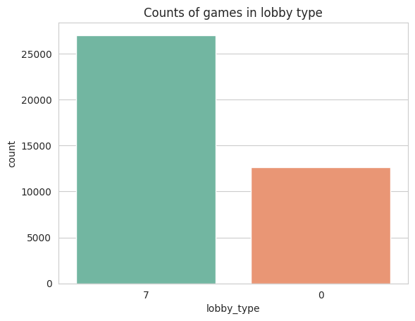
# Create a countplot with a custom color palette
sns.countplot(data=train_data, x='lobby_type', order=train_data['lobby_type'].value_counts().index, palette='Set2');

# Add a title to the plot
plt.title('Counts of games in lobby type');

# Show the plot
plt.show()
# Create a countplot with the 'Set2' color palette for game modes
sns.countplot(data=train_data, x='game_mode',
              order=train_data['game_mode'].value_counts().index, palette='Set2')

# Add a title to the plot
plt.title('Counts of games in different modes')

# Show the plot
plt.show()

# Filter the dataset to only include the most common game mode
most_common_game_mode = train_data['game_mode'].value_counts().idxmax()
filtered_train_data = train_data[train_data['game_mode'] == most_common_game_mode]
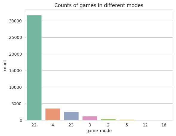
Insight
- Different lobby types and game modes have distinct criteria; therefore, selecting the lobby type and game mode with the highest count ensures a balanced dataset with more consistent datapoints. This approach minimizes potential biases and variations that could arise from considering multiple lobby types and game modes, leading to more reliable predictions and analysis.
Data Preprocessing
Feature Transformation
# remove lobby_type with lower counts
train_y['lobby_type'] = train_data['lobby_type']
train_data = train_data[train_data['lobby_type'] == 7]
test_data = test_data[test_data['lobby_type'] == 7]
train_y = train_y[train_y['lobby_type'] == 7]
# remove game_mode with lower counts
train_y['game_mode'] = train_data['game_mode']
train_data = train_data[train_data['game_mode'] == 22]
test_data = test_data[test_data['game_mode'] == 22]
train_y = train_y[train_y['game_mode'] == 22]
# drop lobby_type and game_mode for train_y
train_y = train_y.drop(columns=['lobby_type', 'game_mode'])
# mapping win and lose values
train_y = train_y['radiant_win'].map({True: 1, False:0})
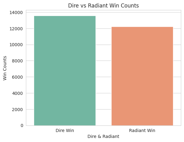
# Get the unique values of 'radiant_win' column
unique_vals = train_y.reset_index()['radiant_win'].unique()
# Get the count of win for each unique value of 'radiant_win'
win_counts = train_y.reset_index()['radiant_win'].value_counts()
# Create a bar plot with the 'Set2' color palette for Dire and Radiant wins
sns.barplot(x=unique_vals, y=win_counts, palette='Set2')
# Set the x-axis tick labels to 'Dire Win' and 'Radiant Win'
plt.xticks([0, 1], labels=['Dire Win', 'Radiant Win'])
# Add labels to the x- and y-axes and a title to the plot
plt.xlabel('Dire & Radiant')
plt.ylabel('Win Counts')
plt.title('Dire vs Radiant Win Counts')
# Show the plot
plt.show()
Feature Engineering
# combing all individual character features into a team based features
feature_names = train_data.columns
num = []
for y in range(24):
    for i in [feature_names[feature_names.str.contains("r"+str(i)) == True] for i in range(1,6)]:
        num.append(i[y])
    col = num[0].split("_")[1]
    train_data['r_'+col] = train_data[num].sum(axis=1)
    test_data['r_'+col] = test_data[num].sum(axis=1)

    # dropping individual features
    train_data.drop(columns=num, inplace=True)
    test_data.drop(columns=num, inplace=True)
    num = []

for y in range(24):
    for i in [feature_names[feature_names.str.contains("d"+str(i)) == True] for i in range(1,6)]:
        num.append(i[y])
    col = num[0].split("_")[1]
    train_data['d_'+col] = train_data[num].sum(axis=1)
    test_data['d_'+col] = test_data[num].sum(axis=1)

    # dropping individual features
    train_data.drop(columns=num, inplace=True)
    test_data.drop(columns=num, inplace=True)
    num = []
Feature Selection
# what features to be used
to_load = (['r_kills', 'r_deaths', 'r_assists', 'r_denies', 'r_lh', 'r_gold',
            'd_kills', 'd_deaths', 'd_assists', 'd_denies', 'd_lh', 'd_gold'])
train_X = train_data[to_load]
test_X = test_data[to_load]

# reduced the datapoints for the interest of runtime and
# to show the significance of the models
feature_names = train_X.columns
train_sample = int(train_X.shape[0]/2)
test_sample = int(test_X.shape[0]/2)

# getting sample size
train_X = train_X.sample(train_sample, random_state=3)
train_y = train_y.sample(train_sample, random_state=3)
test_X = test_X.sample(test_sample, random_state=3)
train_X
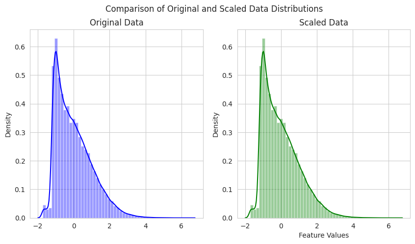
Data Scaling
# Scaling
scaler = StandardScaler()
train_X_scaled = scaler.fit_transform(train_X)
test_X_scaled = scaler.fit_transform(test_X)
Final Data
# scaled data
train_X_scaled # for train value
test_X_scaled # for test value

# original data
train_X # for train value
test_X # for test value

# output to csv
train_X.to_csv('train_X.csv')
test_X.to_csv('test_X.csv')
train_y.to_csv('train_y.csv')
RESULTS AND DISCUSSION
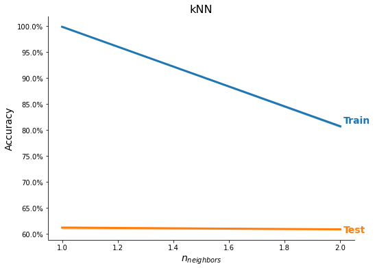
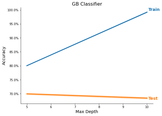
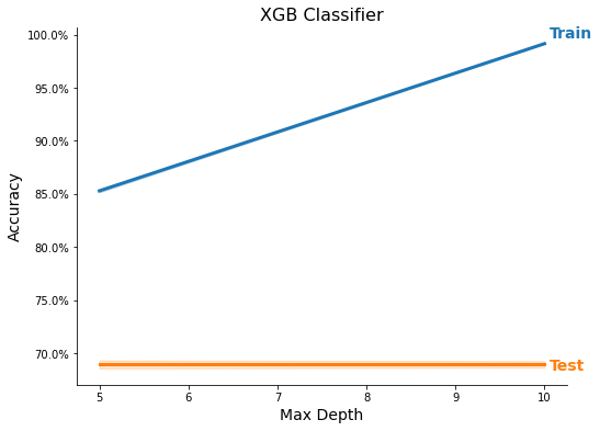
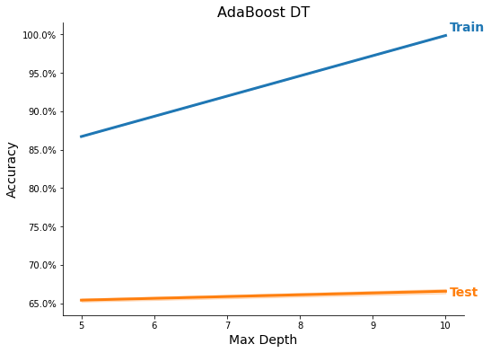
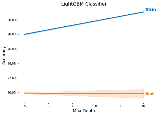
Auto ML Simulation
# Select methods
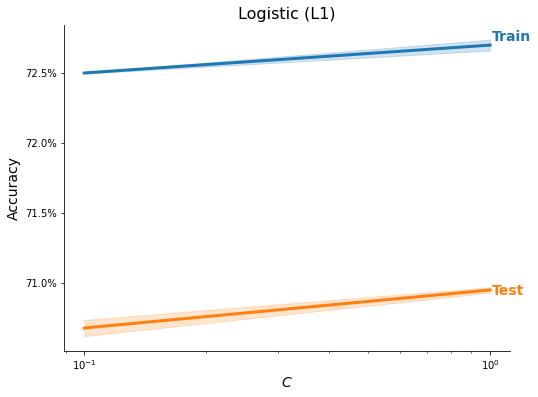
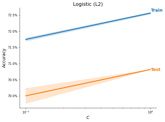
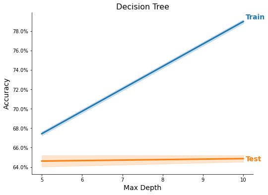
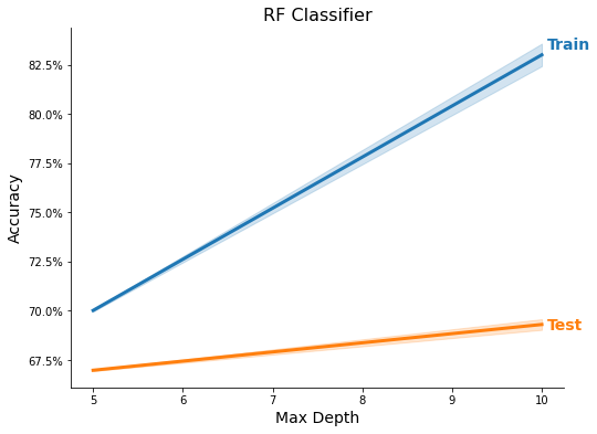
methods = ['kNN', 'Logistic (L1)', 'Logistic (L2)', 'Decision Tree',
'RF Classifier', 'GB Classifier', 'XGB Classifier',
'AdaBoost DT', 'LightGBM Classifier', 'CatBoost Classifier']
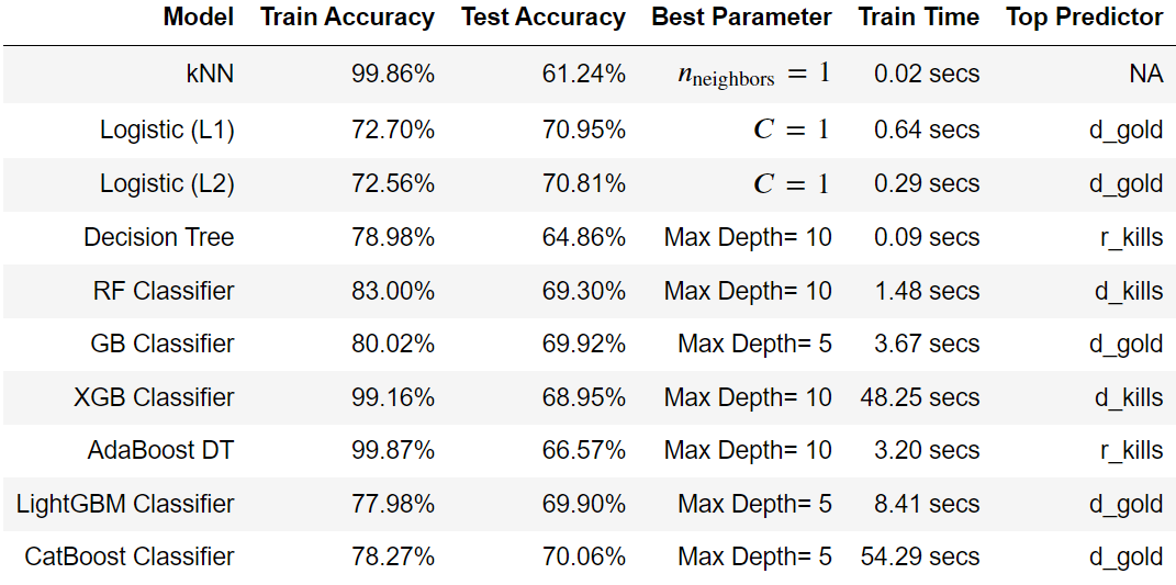
# Perform training and testing
ml_models = MLModels.run_classifier(
train_X_scaled, train_y, feature_names, task='C',
use_methods=methods, n_trials=2, tree_rs=3, test_size=0.20,
n_neighbors=list(range(1, 3)),
C=[1e-1, 1],
max_depth=[5, 10])
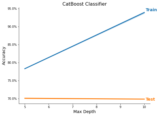
res = MLModels.summarize(ml_models, feature_names,
show_plot=True, show_top=True)
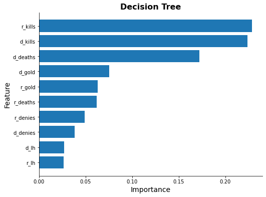
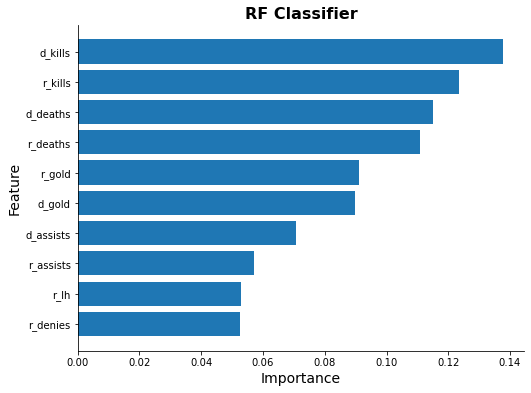
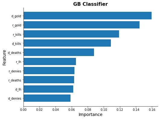
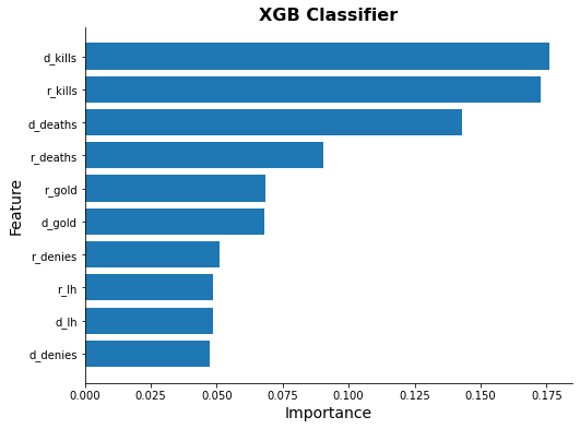
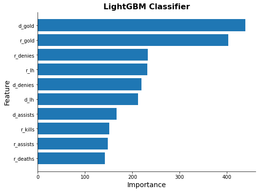
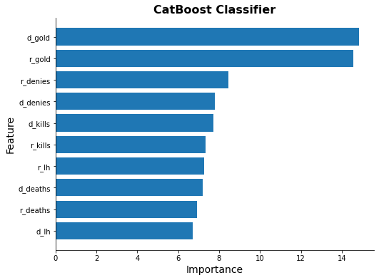
Feature Importance
for model_name in methods[3:]:
    try:
        ax = ml_models[model_name].plot_feature_importance(feature_names)
        ax.set_title(model_name, fontsize=16, weight="bold")
    except Exception as e:
        print(model_name, e)
Light GBM Classifier Simulation
# reduced params range based from previous multiple trials
tune_model(train_X_scaled, train_y, 'Classification', 'LightGBM Classifier',
           params={'max_depth': [25, 50],
                   'n_estimators': [150, 200],
                   'learning_rate': [0.1, 0.2]},
           n_trials=2, tree_rs=3)
| Model | Accuracy | Best Parameter |
|---|---|---|
| LightGBM Classifier | 69.41% | {'max_depth': 25, 'n_estimators': 200, 'learning_rate': 0.1} |
| Classifier | LGBMClassifier(max_depth=25, n_estimators=200, random_state=3) | |
| acc | 69.41 | |
| std | 0.0013953488372092648 | |
Bayesian Optimization Simulation
In this project, we demonstrated the use of Bayesian optimization as a function optimization package by optimizing three hyperparameters of the LightGBM classifier. This was done to show how Bayesian optimization can improve the accuracy of a machine learning model by finding the optimal combination of hyperparameters.
The function to be optimized
def lgb_cv(num_leaves, max_depth, min_data_in_leaf):
    params = {
        "num_leaves": int(num_leaves),
        "max_depth": int(max_depth),
        "learning_rate": 0.5,
        'min_data_in_leaf': int(min_data_in_leaf),
        "force_col_wise": True,
        'verbose': -1,
        "metric" : "auc",
        "objective" : "binary",
    }

    lgtrain = lightgbm.Dataset(train_X_scaled, train_y)
    cv_result = lightgbm.cv(params,
                       lgtrain,
                       200,
                       early_stopping_rounds=200,
                       stratified=True,
                       nfold=5)
    return cv_result['auc-mean'][-1]
The optimizer function
def bayesian_optimizer(init_points, num_iter, **args):
    lgb_BO = BayesianOptimization(lgb_cv, {'num_leaves': (100, 200),
                                           'max_depth': (25, 50),
                                           'min_data_in_leaf': (50, 200)
                                           })
    lgb_BO.maximize(init_points=init_points, n_iter=num_iter, **args)
    return lgb_BO

results = bayesian_optimizer(10,10)
| iter | target | max_depth | min_data_in_leaf | num_leaves |
|---|---|---|---|---|
| 1 | 0.7859 | 49.98 | 128.7 | 115.4 |
| 2 | 0.7796 | 42.94 | 68.67 | 190.1 |
| 3 | 0.7784 | 28.36 | 57.48 | 107.0 |
| 4 | 0.7869 | 30.55 | 134.1 | 150.3 |
| 5 | 0.7892 | 36.73 | 162.4 | 187.3 |
| 6 | 0.7866 | 31.26 | 195.5 | 165.7 |
| 7 | 0.7804 | 37.51 | 75.45 | 175.9 |
| 8 | 0.7848 | 45.02 | 123.7 | 153.1 |
| 9 | 0.7842 | 33.06 | 124.2 | 109.2 |
| 10 | 0.7884 | 39.39 | 164.4 | 142.8 |
| 11 | 0.7882 | 39.39 | 165.1 | 143.5 |
| 12 | 0.7881 | 50.0 | 179.0 | 100.0 |
| 13 | 0.7895 | 50.0 | 200.0 | 200.0 |
| 14 | 0.7892 | 25.0 | 186.1 | 200.0 |
| 15 | 0.7882 | 25.0 | 165.9 | 113.4 |
| 16 | 0.7876 | 25.0 | 138.8 | 200.0 |
Train Iterations with the optimized parameters
def lgb_train(num_leaves, max_depth,  min_data_in_leaf):
    params = {
        "num_leaves": int(num_leaves),
        "max_depth": int(max_depth),
        "learning_rate": 0.5,
        'min_data_in_leaf': int(min_data_in_leaf),
        "force_col_wise": True,
        'verbose': -1,
        "metric": "auc",
        "objective": "binary",
    }

    x_train, x_val, y_train, y_val = train_test_split(
        train_X_scaled, train_y, test_size=0.2, random_state=3)
    lgtrain = lightgbm.Dataset(x_train, y_train)
    lgvalid = lightgbm.Dataset(x_val, y_val)
    model = (lightgbm.train(params, lgtrain, 200, valid_sets=[lgvalid],
                            early_stopping_rounds=200, verbose_eval=False))
    prediction_val = model.predict(
        test_X_scaled, num_iteration=model.best_iteration)
    return prediction_val, model
Optimize Simulation Results
# 5 runs of the prediction model and get mean values.
optimized_params = results.max['params']
prediction_val1, _ = lgb_train(**optimized_params)
prediction_val2, _ = lgb_train(**optimized_params)
prediction_val3, _ = lgb_train(**optimized_params)
prediction_val4, _ = lgb_train(**optimized_params)
prediction_val5, model = lgb_train(**optimized_params)
y_pred = ((prediction_val1 + prediction_val2 +b
           prediction_val3 + prediction_val4 +
           prediction_val5)/5)
df_result = pd.DataFrame(
    {'Radiant_Win_Probability': y_pred})
df_result.sort_values(by='Radiant_Win_Probability', ascending=False).head()
| Match ID Hash | Radiant Win Probability |
|---|---|
| 895 | 0.993668 |
| 1617 | 0.990840 |
| 1752 | 0.989719 |
| 245 | 0.987856 |
| 2742 | 0.986903 |
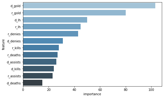
feature_importance = (pd.DataFrame({'feature': train_X.columns,
                                   'importance': model.feature_importance()})
                      .sort_values('importance', ascending=False))
plt.figure(figsize=(8, 5))
sns.barplot(x=feature_importance.importance,
            y=feature_importance.feature, palette=("Blues_d"))
plt.show()
CONCLUSION AND RECOMMENDATION
The nature of Dota2 as a game with only one winner and one loser makes it a suitable problem for machine learning prediction. However, real-time predictions during a game can be challenging due to the need for specific information per minute. In this project, we used multiple models to determine the most suitable approach for predicting Dota2 game outcomes. Additionally, hyperparameter tuning was performed to optimize model performance, with Bayesian optimization being the preferred method due to its efficiency when dealing with expensive-to-evaluate functions like LightGBM.
While the use of Bayesian optimization for hyperparameter tuning might not be as significant for small datasets or simple models, it becomes essential when dealing with enormous datasets where grid search may not be economically feasible. Therefore, the use of Bayesian optimization can improve the efficiency of the hyperparameter search process.
To further enhance prediction accuracy, we recommend the use of time-series machine learning models to provide real-time forecasting during the game. Such models can take into account the changing dynamics of the game and provide more accurate predictions.
In conclusion, this notebook provides valuable insights into Dota2 as a growing Esport and demonstrates how different machine learning models can be used to predict game outcomes. By leveraging hyperparameter optimization techniques like Bayesian optimization and considering time-series models for real-time prediction, we can improve the accuracy of our predictions and gain a deeper understanding of Dota2 as an Esport.
REFERENCES
[1] Dota 2. (n.d.). https://www.dota2.com/home
[2] Staff, T. G. H. (2022, September 7). What Makes Dota 2 So Successful. The Game Haus. https://thegamehaus.com/dota/what-makes-dota-2-so-successful/2022/04/02/
[3] mlcourse.ai: Dota 2 Winner Prediction Kaggle. (n.d.). https://www.kaggle.com/competitions/mlcourse-dota2-win-prediction/overview
[4] Dota 2 5v5 - Red vs Blue by dcneil on. (2013, October 9). DeviantArt. https://www.deviantart.com/dcneil/art/Dota-2-5v5-Red-vs-Blue-406091855
[5] mlcourse.ai: Dota 2 Winner Prediction Kaggle. (n.d.-b). https://www.kaggle.com/competitions/mlcourse-dota2-win-prediction/data
[6] Dota 2 Wiki. (n.d.). https://dota2.fandom.com/wiki/Dota_2_Wiki
[7] fmfn, F. (n.d.). GitHub - fmfn/BayesianOptimization: A Python implementation of global optimization with gaussian processes. GitHub. https://github.com/fmfn/BayesianOptimization
[8] Natsume, Y. (2022, April 30). Bayesian Optimization with Python - Towards Data Science. Medium. https://towardsdatascience.com/bayesian-optimization-with-python-85c66df711ec
- Note: the mltools of Prof Leodegario U. Lorenzo II and feedbacks of our Mentor Prof Gilian Uy and also the other professors significantly made this notebook very cool!