
Magic the Gathering: Winning Not by What (Colors) You Play, but by How You Play
Published:

Executive Summary
In this report, we explore the world of spectacularly-designed cards with gothic creatures, insightful texts, and five distinct colors - the world of Magic the Gathering (MTG), which is dubbed as the world’s most complex game. [3]
We set out to identify the MTG Color that will set the player so far out in the lead from his opponents.
We evaluated the distinct colors, various types, different powers, diverse toughness, varying converted mana cost, distinctive keywords/abilities, and Elder Dragon Highlander Recommendations (EDHREC) rank.
Our data processing, analysis, and visualization results reveal that no color enjoys a compelling advantage in singlehandedly emerging victorious in MTG. We found that no color monopolizes staging the optimal or winning MTG play.
The colors have and thrive in uniqueness, making it difficult to compare them. Ultimately, it’s not about what (colors) you play, but how you play MTG.
We also note that MTG has inspired the publishing of several books bearing the MTG title and has given rise to the MTG genre.
Problem Statement
**Which Color of Magic The Gathering Should You Play to Win?**We will analyze the different colors of the MTG Cards and find out whether one has a striking advantage to win the MTG Gameplay.
Introduction
A Brief History of MTG: [4]
Mathematician Richard Garfield created MTG on August 5, 1993.
The first core set, Alpha, contained 295 cards. Now, MTG has more than a hundred expansion sets. In addition, new game formats were invented (e.g., Magic Arena Digital Card Game) and highly successful video games (e.g., Duels of the Planeswalkers Games).
MTG Professional Circuit involves thousands of players and hundreds of thousands of viewers. MTG has over 23,000 unique cards and over 20 billion cards printed.
Lore and History of the MTG Multiverse [4]
MTG is a fantasy battle of players who take on the roles of Planeswalkers – powerful beings able to hop between the many planes of reality within the MTG Multiverse.
As a Planeswalker travels through the metaphysical journey, he visits places, meets creatures, and discovers spells. The player’s deck is a collection of memories of the Planeswalker’s experiences.
The MTG Colors Each color is focused on a different gameplay style: [4]
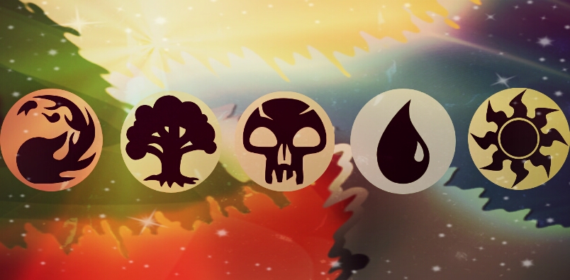
1) White is about Light and Life
White focuses on healing players or protecting creatures on the board and has powerful angelic creatures and defensive spells.
Plains produce white mana.
2) Blue is about Control and Strategy
Blue decides and dictates the flow of the battle, counters the spells cast by the opponent, and prevents them from doing things or drawing more cards.
Islands produce blue mana.
3) Black is about Death and Pain
Black kills creatures, harms enemies, or harms the player himself. Black sees all lives, including the player, as a resource that can be spent to accomplish the end goal.
Swamps produce black mana.
4) Red is about Anger and Damage
Red is the most aggressive, and Red spells are about doing as much damage as fast as possible. Red doesn’t care too much about being subtle or crafty. It’s all about attacking.
Mountains produce red mana.
5) Green is about Growth and Regeneration
Green accelerates land and grows huge creatures. Green helps a player race ahead of his opponent by generating more mana or playing many creatures very quickly.
Forests produce green mana.
6) Colorless is devoid of the traits of the main five colors
Ancient and plane-destroying Eldrazi needs it.
Colorless mana is produced by wastes.
General Rules of Play [4]
Each player:
1) Holds a deck of 60 cards or more. The usual number is 60, but the players are sometimes allowed to exceed that number.
2) Can hold up to 4 copies of any named card (except Lands).
3) Can hold as many Lands as possible.
4) Starts with 20 Life Points.
5) Aims to reduce opponent’s Life Points to 0.
Gameplay Formats [4]
The following are the popular gameplay formats of MTG.
1) Kitchen Table Magic - Any card is allowed.
2) Standard - Only cards from the recent 3 or 4 sets are allowed, meaning sets rotate in and out of Standard. Standard is a rotating format. Any printing of a current Standard card may be used. The current sets in Standard are listed here
3) Modern - All cards in any set are printed from 2003 and onwards (the 8th edition and later) unless they are specifically on the ban list. Unlike Standard, Modern is a non-rotating format.
4) Legacy/Vintage - Allows cards from most of MTG’s history, including the immensely powerful, extremely expensive cards like the Power 9 or the Duel Lands (USD 1,000 - USD 40,000).
5) Draft - Random, casual, and fun format involving a group of 8 players buying three booster packs each. Each booster pack contains ten random cards. They each open their booster packs, take 1 card and pass the pack to the next until each player’s three booster packs have been distributed evenly to all other players. They then build a deck from the cards they take and then play.
6) Commander - Multiplayer format where players pick a Legendary Creature as Commander and then build a 100-card deck. Each card should be unique and contain the same mana colors as the Commander. Each player starts with 40 Life Points.
Other gameplay formats are Oathbreaker, Pauper, Planechase, and Archenemy.
Data Description
We used the following data in this report: [7]
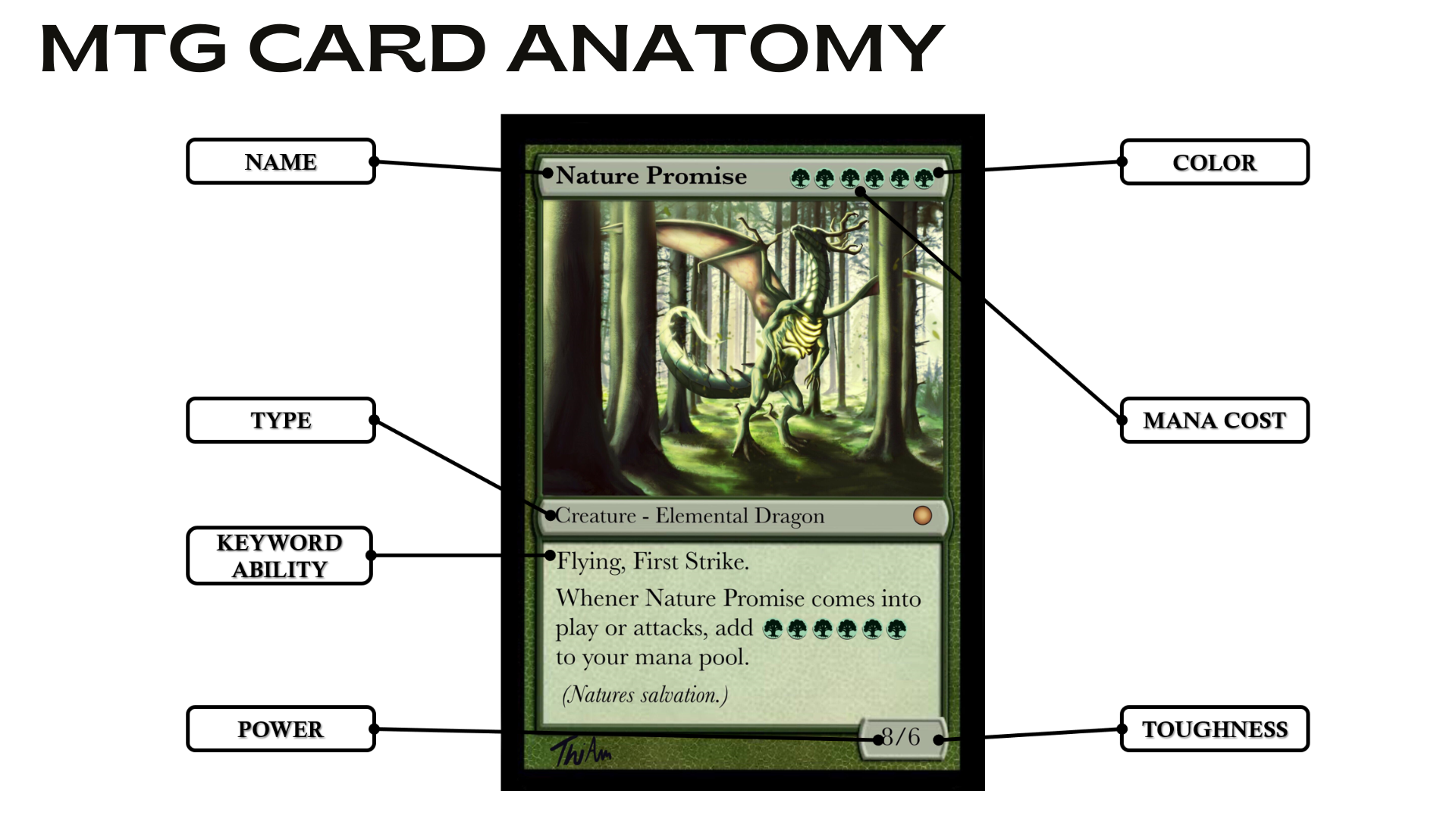
1) Name - The name of the MTG card printed on its upper left corner, always considered to be the English version of its name, regardless of printed language.
2) Color - A basic property of MTG cards directly related to the core of MTG’s mana system and overall strategy. There are five colors, sequenced white ({W}), blue ({U}), black ({B}), red ({R}), and green ({G}); this arrangement is called the “color pie” or “color wheel”.
3) Types - Is a characteristic found on every MTG card. MTG cards typically have one or more of either the permanent types: land, creature, artifact, enchantment, and planeswalker, or of the non-permanent spell types: instant and sorcery.
4) Power - Is the first number printed before the slash on the lower right-hand corner of creature cards. This is the amount of damage it deals in combat to the opposing creature’s toughness, the opposing player’s life total, or the opposing planeswalker’s loyalty.
5) Toughness - Toughness is the number printed after the slash at the bottom right corner of a creature. It is the amount of damage needed to destroy it. If the number becomes equal to or less than 0 at any time, it is put into its owner’s graveyard as a state-based action.
6) Converted Mana Cost - The converted mana cost of an object is determined by counting the total amount of mana in its mana cost, regardless of color.
7) Keyword Ability - A keyword ability is a word or words that represents a piece of rules text describing an ability present on a card.
8) Elder Dragon Highlander Recommendations (EDHREC) Ranking - EDHREC’s ranking of the most popular cards in Commander decks, as submitted by users in a crowdsourced repository.
9) Printings - The number of prints of an MTG card. The higher the number of prints, the more popular the MTG card is.
Data Processing & Methodology
Importing Libraries
import pandas as pd
import numpy as np
import seaborn as sns
import sqlite3

import matplotlib.pyplot as plt
plt.rcParams["figure.figsize"] = (12,6)
Loading the MTG JSON file
All Printings JSON
abs_filepath = 'AllPrintings.json'
df = pd.read_json(abs_filepath)
df1 = pd.json_normalize(df['data'][2:])
df_all = pd.DataFrame()
for i in range(len(df1.index)):
    df_all = pd.concat([df_all, pd.DataFrame.from_dict(df1['cards'][i])])
display(df_all.head())
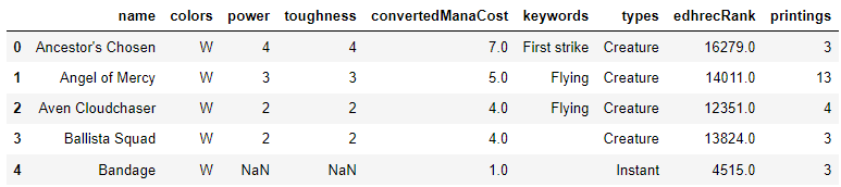
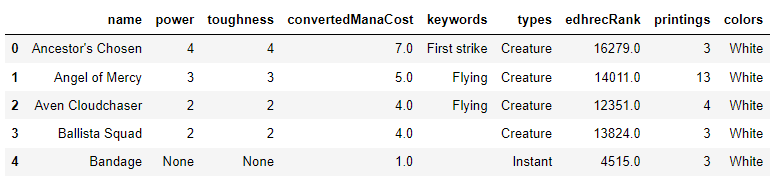
To answer the question: Is the game balanced? We will need only a few columns out of a total of 64 columns.
df_data = df_all.copy()
df_data = df_data[['name', 'colors', 'power', 'toughness',
                   'convertedManaCost', 'keywords', 'types',
                   'edhrecRank', 'printings']]
display(df_data.head())
Some of the values of columns are lists. So we will convert it first into a string before we can save it into the database.
df_data['colors'] = [','.join(map(str, l)) for l in df_all['colors']]
df_data['types'] = [','.join(map(str, l)) for l in df_all['types']]
df_data['printings'] = [(','.join(map(str, l))).count(',') +1
                        for l in df_all['printings']]
df_all['keywords'] = df_all['keywords'].replace(np.nan, "")
df_data['keywords'] = [','.join(map(str, l)) for l in df_all['keywords']]
display(df_data.head())
Deck JSON
df_deck_json = json.load(open('DeckList.json'))
df_deck = pd.DataFrame(df_deck_json['data'])
Saving to Database
conn = sqlite3.connect('mtg.db')
cursor = conn.cursor()
cursor.executescript("""
CREATE TABLE IF NOT EXISTS cards(
    colors TEXT,
    name TEXT,
    convertedManaCost FLOAT,
    power TEXT,
    toughness TEXT,
    types TEXT,
    keywords TEXT,
    edhrecRank FLOAT,
    printings FLOAT
);
CREATE TABLE IF NOT EXISTS decks(
    code TEXT,
    filename TEXT,
    name TEXT,
    releaseDate TEXT,
    type TEXT
);
""");

df_data.to_sql('cards', con=conn, if_exists='replace', index=False)
df_deck.to_sql('decks', con=conn, if_exists='replace', index=False);
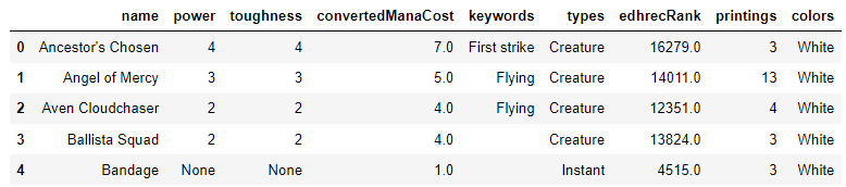
Loading from Database
All Printings
sql = """
SELECT *
FROM cards
"""
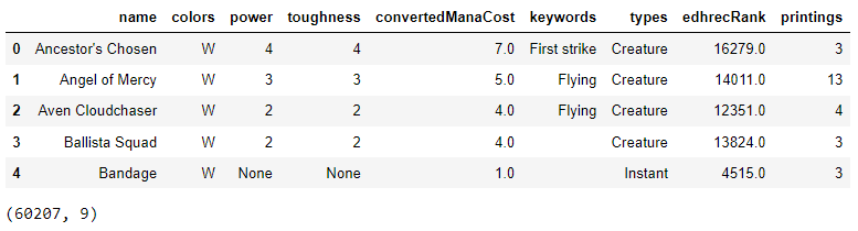
df_sql = pd.read_sql(sql, conn)
display(df_sql.head())
print(df_sql.shape)
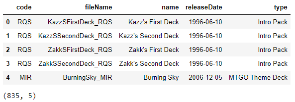
Deck List
sql = """
SELECT *
FROM decks
"""
df_decklist = pd.read_sql(sql, conn)
display(df_decklist.head())
print(df_decklist.shape)
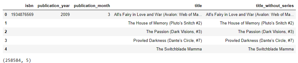
Good Reads
sql = """
SELECT *
FROM books
"""
df_books = pd.read_sql(sql, conn)
display(df_books.head())
print(df_books.shape)
Removing duplicated rows
print(f'Total number of duplicated rows: {df_sql.duplicated().sum()}')
Duplicated rows come from the fact that cards that have alternate art forms/reprinted are entered as separate rows.
df_sql.drop_duplicates(inplace=True)
print(f'Total number of duplicated rows: {df_sql.duplicated().sum()}')
print(f'Total number of unique rows    : {df_sql.shape[0]}')
This value is corroborated by the estimated value (more than 20,000) posted on in the Magic: The Gathering Wiki page. [7]
Categorizing Card Colors
Cards can have White (W), Blue (U), Black (B), Red (R), Green (G), colorless, or any combination of the color mentioned. For the simplicity of analysis, we will categorize any combination of colors into the Multicolor category.
df_sql['colorstr'] = 'Multicolor'
df_sql.loc[df_sql['colors'] == 'W', 'colorstr'] = 'White'
df_sql.loc[df_sql['colors'] == 'U', 'colorstr'] = 'Blue'
df_sql.loc[df_sql['colors'] == 'B', 'colorstr'] = 'Black'
df_sql.loc[df_sql['colors'] == 'R', 'colorstr'] = 'Red'
df_sql.loc[df_sql['colors'] == 'G', 'colorstr'] = 'Green'
df_sql.loc[df_sql['colors'] == '', 'colorstr'] = 'Colorless'
df_sql.drop(columns='colors', inplace=True)
df_sql.rename(columns={'colorstr': 'colors'}, inplace=True)
display(df_sql.head())
Categorizing Card Types
Magic cards have either of the Card Type: Artifact, Creature, Enchantment, Instant, Land, Planeswalker, or Sorcery. Some cards may include types that are not part of the primary seven types or a combination of those seven. Those card types will be categorized as Others.
df_sql.loc[(df_sql['types'] != 'Artifact')
            & (df_sql['types'] != 'Creature')
            & (df_sql['types'] != 'Enchantment')
            & (df_sql['types'] != 'Instant')
            & (df_sql['types'] != 'Land')
            & (df_sql['types'] != 'Planeswalker')
            & (df_sql['types'] != 'Sorcery'), 'types'] = 'Others'
display(df_sql.head())
Exploratory Data Analysis
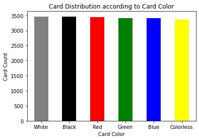
Color Distribution
# This will be for plotting
color_map = {'White': 'gray', 'Blue': 'blue', 'Black': 'black', 'Red': 'red',
             'Green': 'green', 'Colorless': 'yellow', 'Multicolor': 'orange'}

# Remove Multicolor since its represents multiple colors
df_color = df_sql['colors'].value_counts()
df_color = df_color[(df_color.index != 'Multicolor')]

# Plot
df_color.plot.bar(color=[color_map[key] for key in list(df_color.index)])
plt.xticks(rotation=0, horizontalalignment="center")
plt.title('Card Distribution according to Card Color')
plt.xlabel('Card Color')
plt.ylabel('Card Count')
plt.show()
# To avoid error in loading the correct size of the next figures
import matplotlib.pyplot as plt
plt.rcParams["figure.figsize"] = (12,6)
color_diff = (df_color.max() - df_color.min()) / df_color.min()
print(f'The highest card count is only {color_diff*100:.2f}%'
      f'higher than the lowest card count.')
Insight:
- Cards are balanced in terms of color representation.
Type Distribution
Overall
# Remove others since its a aggregation of multiple non-basic types
df_type = df_sql['types'].value_counts()
df_type = df_type[(df_type.index != 'Others')]

# Plot
df_type.plot.bar()
plt.xticks(rotation=0, horizontalalignment="center")
plt.title('Card Distribution according to Card Type')
plt.xlabel('Card Type')
plt.ylabel('Card Count')
plt.show()
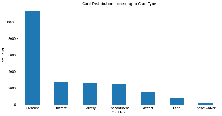
creature_pct = df_type.max() / df_type.sum()
print(f'Creature type composes {creature_pct*100:.2f}'
      f'% of the total card count.')
Insight:
- Cards are mostly creature-type.
Per Card Color
df_ct = pd.crosstab(df_sql['colors'],
                    df_sql['types']).reindex(list(color_map.keys()))

for card_type in list(df_sql['types'].unique()):
    df_ct[card_type].plot(kind='bar', color=list(color_map.values()))
    plt.xticks(rotation=0, horizontalalignment="center")
    plt.title(f'Distribution of {card_type} according to Card Color')
    plt.xlabel('Card Color')
    plt.ylabel(f'No. of Card with {card_type} type')
    plt.show()
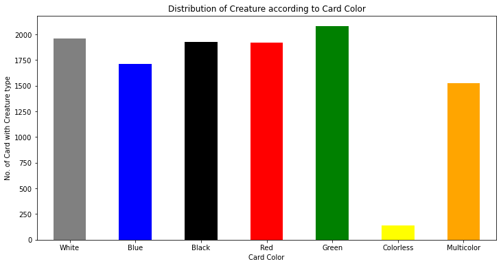
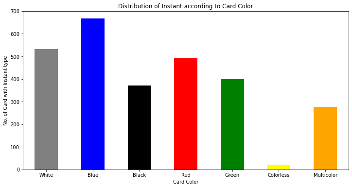
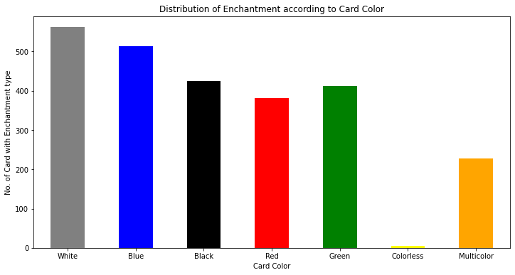
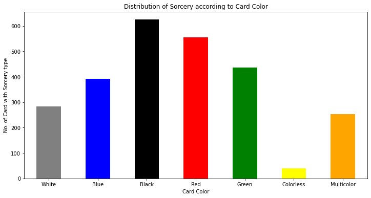
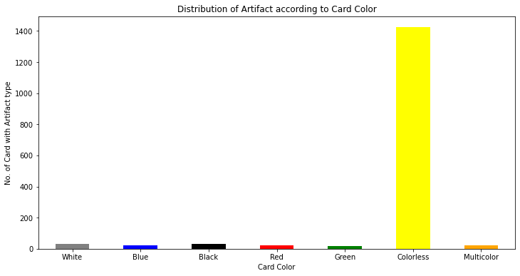
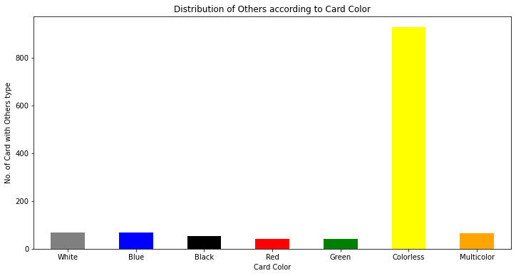
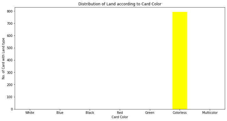
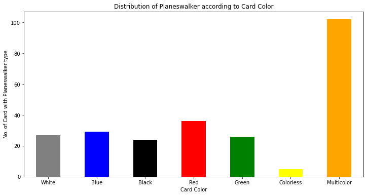
Insights:
- The five primary card colors have almost the same number of
Creaturecards exceptBlue.CreatureswithColorlessare rare. Instantcards are mostlyBlue.Enchantmentcards are mostlyWhitebut are closely followed byBlue.Sorcerycards are mostlyBlackbut are closely followed byRed.ArtifactandOthercards are almost allColorless.- All
Landcards areColorless. - Majority of
Planeswalkercards areMulticolor.
Power Analysis
Possible Power Values
print(df_sql['power'].unique())
df_power = df_sql.copy()
card_cnt = df_sql.shape[0]
df_power = df_power[df_power['power'].notna()]
card_power_cnt = df_power.shape[0]
print(f'Total cards                 : {card_cnt}')
print(f'Total cards with Power value: {card_power_cnt}')
Some cards don’t have power values, represented in the data as None. Therefore, only cards with power values will be compared.
Variable Power Values
print(df_power['power'].unique())
df_power = df_power[(df_power['power'] != '*') & (df_power['power'] != '2+*')
                    & (df_power['power'] != '1+*')
                    & (df_power['power'] != '-1')
                    & (df_power['power'] != '?')
                    & (df_power['power'] != '+2')
                    & (df_power['power'] != '+1')
                    & (df_power['power'] != '∞')
                    & (df_power['power'] != '*²')
                    & (df_power['power'] != '+3')
                    & (df_power['power'] != '+4')
                    & (df_power['power'] != '+0')
                    & (df_power['power'] != '99')]
card_power_static_cnt = df_power.shape[0]
print(f'Card count with static power value  : {card_power_static_cnt}')
print(f'Card count with variable power value: '
      f'{card_power_cnt-card_power_static_cnt}')
The power value may be a static float value or some variable value. Only static values will be compared. Variable power value would be impossible to compare outside the game it is played.
df_power['power'] = df_power['power'].astype(float)
print(df_power['power'].unique())
Variable Power Examples and Explanation
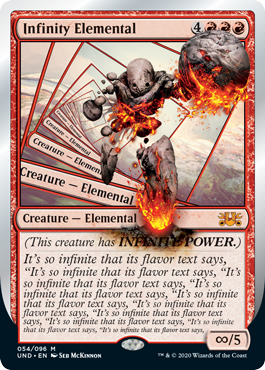
- An example of an MTG Card with ∞ (infinity) is
Infinity Elemental. It has infinite power such that gaining or losing power doesn’t affect it, but it can still be affected by an ability that sets the power to a specific value.
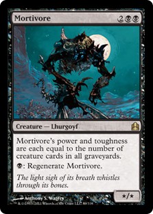
- An example of an MTG card with * (asterisk) is
Mortivore. The value of its power depends on the number of creatures in all graveyards. Other cards, such as *², act similarly but squared. Asterisk indicates that its power depends on some in-game variable (e.g., graveyard card counts, player hand card count).
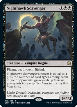
- An example of an MTG card with 1+* (base number + asterisk) is
Nighthawk Scavenger. Its power has a base value of 1, then added to the number of card types among cards in the opponent’s graveyard. Base number + asterisk indicates a base value for power but is added with a power value dependent on some in-game variable.
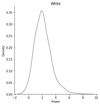
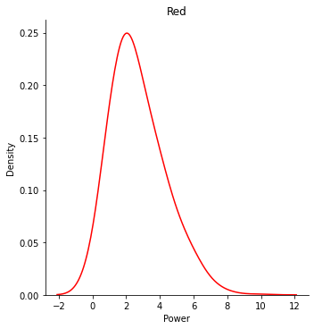
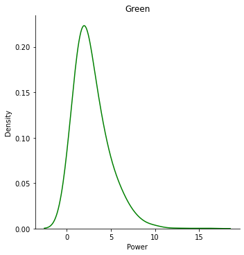
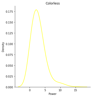
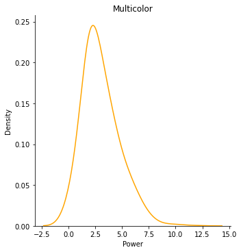
Static Power Values
These are cards with power values represented by a float, e.g., 1.0, 2.5.
unique_color = list(df_power['colors'].unique())
color_mean_value = {}
for color in unique_color:
sub_df = df_power.copy()
sub_df = sub_df[sub_df['colors'] == color]
mean_power = sub_df['power'].mean()
color_mean_value[color] = mean_power
# Plot each distribution (per color)
sns.displot(sub_df['power'], kind='kde', bw_adjust=2,
color=color_map[color])
plt.title(color)
plt.xlabel('Power')
plt.show()
print(f"Average Power of {color} is {sub_df['power'].mean():.2f}\n\n")
# Overlaying all distribution plots
sns_palette = [color_map[key] for key in list(df_power['colors'].unique())]
sns.displot(data=df_power, x='power', hue='colors', kind='kde',
bw_adjust=2, height=8, aspect=1, palette=sns_palette)
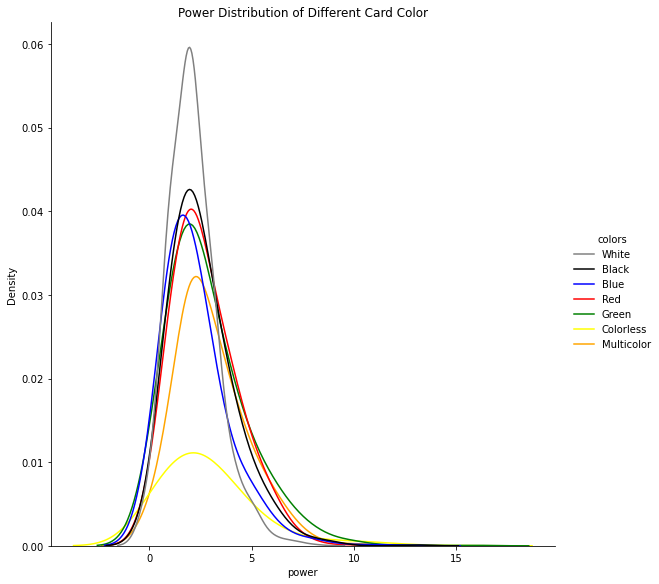
plt.title('Power Distribution of Different Card Color')
plt.show()
# Comparing the different means
sr_mean_power = pd.Series(color_mean_value)
sr_mean_power.plot.bar(color=[color_map[key]
                              for key in list(sr_mean_power.index)])
plt.xticks(rotation=0, horizontalalignment="center")
plt.title('Mean Power of Each Card Color')
plt.xlabel('Card Color')
plt.ylabel('Power')
plt.show()
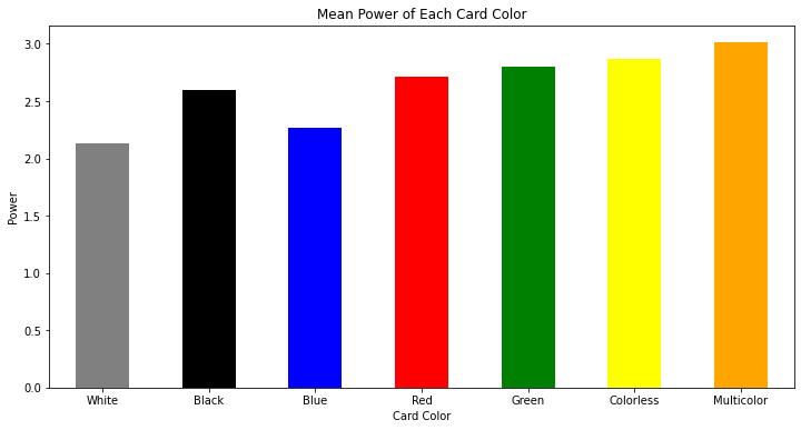
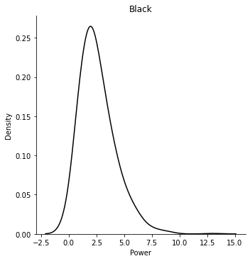
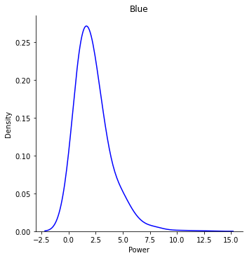
Insights:
- Among all color categories, the highest power comes from
Multicolor(Power: 3.01). - Next highest power is
Black,Red,Green, andColorless(Power: 2.60 - 2.87). WhiteandBluecards have relatively lower average power (Power: 2.13 - 2.27).
Toughness Analysis
Possible Toughness Values
df_sql['toughness'].unique()
df_tough = df_sql.copy()
card_cnt = df_sql.shape[0]
df_tough = df_tough[df_tough['toughness'].notna()]
card_tough_cnt = df_tough.shape[0]
print(f'Total cards                     : {card_cnt}')
print(f'Total cards with Toughness value: {card_tough_cnt}')
Some cards don’t have toughness values represented in the data as None. Therefore, a comparison will only be made to cards with toughness value.
Variable Toughness Values
print(df_tough['toughness'].unique())
df_tough = df_tough[(df_tough['toughness'] != '*')
                    & (df_tough['toughness'] != '2+*')
                    & (df_tough['toughness'] != '7-*')
                    & (df_tough['toughness'] != '-1')
                    & (df_tough['toughness'] != '1+*')
                    & (df_tough['toughness'] != '?')
                    & (df_tough['toughness'] != '*+1')
                    & (df_tough['toughness'] != '99')
                    & (df_tough['toughness'] != '+3')
                    & (df_tough['toughness'] != '+1')
                    & (df_tough['toughness'] != '-0')
                    & (df_tough['toughness'] != '*²')
                    & (df_tough['toughness'] != '+2')
                    & (df_tough['toughness'] != '+4')
                    & (df_tough['toughness'] != '+0')]
card_tough_static_cnt = df_tough.shape[0]
print(f'Card count with static toughness value  : {card_tough_static_cnt}')
print(f'Card count with variable toughness value: '
      f'{card_tough_cnt-card_tough_static_cnt}')
The toughness value may be a static float value or some variable value. Only static values will be compared. Variable toughness value would be impossible to compare outside the game it is played.
df_tough['toughness'] = df_tough['toughness'].astype(float)
print(df_tough['toughness'].unique())
Variable Toughness Examples and Explanation
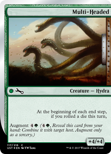
- An example of an MTG Card with +4 (+ number) is
Multi-Headed. This card is an augment card with no toughness value, but the +4 can be added to other cards.
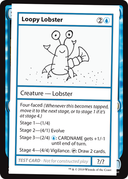
- An example of an MTG card with ? (question mark) is
Loopy Lobster. The value of its toughness evolves through time. Specific values are listed in the card text.
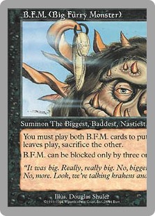
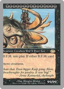
- An example of an MTG card with 99 (large number) is
B.F.M. (Big Furry Monster). It is divided into two cards and can only be played when both are on the playing field. The toughness value is valid, but it has special requirements.
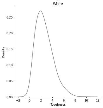
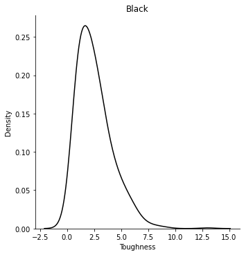
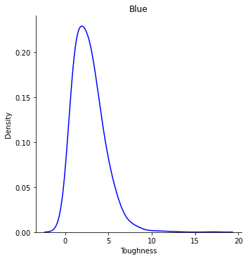
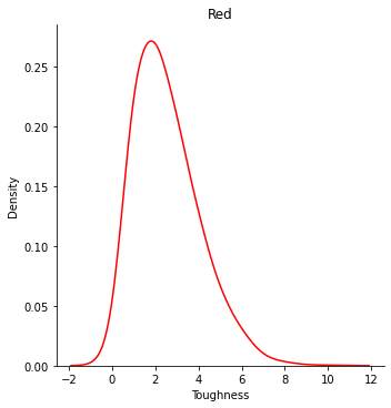
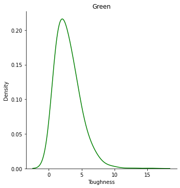
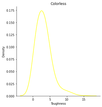
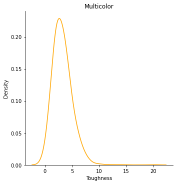
Static Toughness Values
These are cards with toughness values represented by a float, e.g., 1.0, 2.5.
unique_color = list(df_tough['colors'].unique())
color_mean_value = {}
for color in unique_color:
sub_df = df_tough.copy()
sub_df = sub_df[sub_df['colors'] == color]
mean_tough = sub_df['toughness'].mean()
color_mean_value[color] = mean_tough
# Plot each distribution (per color)
sns.displot(sub_df['toughness'], kind='kde', bw_adjust=2,
color=color_map[color])
plt.title(color)
plt.xlabel('Toughness')
plt.show()
print(f"Average Power of {color} is {sub_df['toughness'].mean():.2f}\n\n")
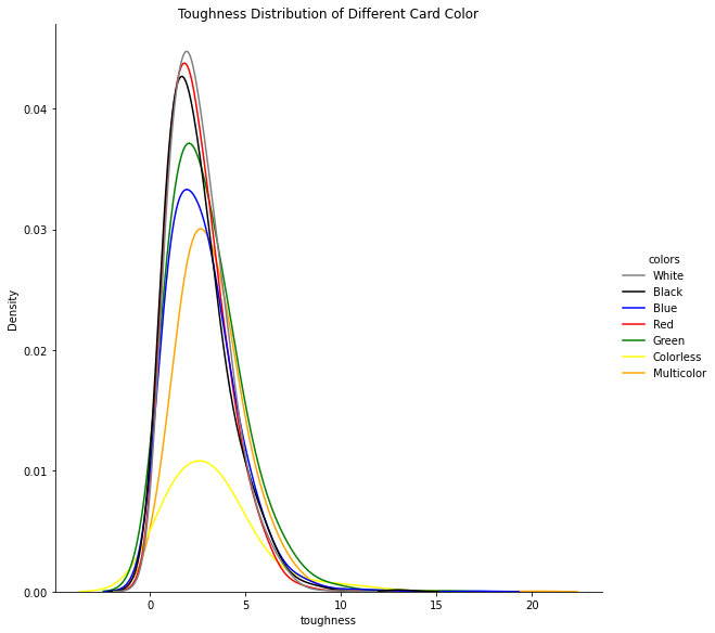
# Overlaying all distribution plots
sns_palette = [color_map[key] for key in list(df_power['colors'].unique())]
sns.displot(data=df_tough, x='toughness', hue='colors', kind='kde',
bw_adjust=2, height=8, aspect=1, palette=sns_palette)
plt.title('Toughness Distribution of Different Card Color')
plt.show()
# Comparing the different means
sr_mean_tough = pd.Series(color_mean_value)
sr_mean_tough.plot.bar(color=[color_map[key]
                              for key in list(sr_mean_tough.index)])
plt.xticks(rotation=0, horizontalalignment="center")
plt.title('Mean Toughness of Each Card Color')
plt.xlabel('Card Color')
plt.ylabel('Toughness')
plt.show()
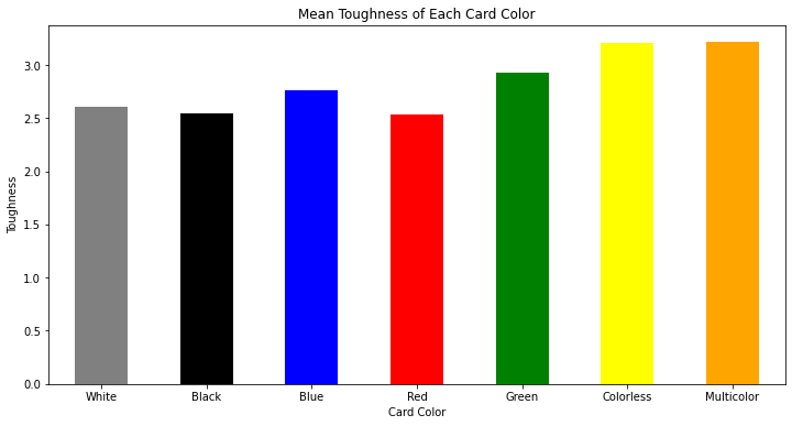
Insights:
- Among all color categories, the highest toughness comes from
ColorlessandMulticolor(Toughness: 3.21 - 3.22). - Next highest toughness is
BlueandGreen(Toughness: 2.76 - 2.93). White,Black, andRedcards have relatively lower average toughness (Toughness: 2.54 - 2.61).
Converted Mana Cost (CMC) Analysis
Overall CMC
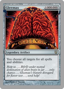
There is an outlier in Converted Mana Cost (CMC). Gleemax card has a CMC of 1000000. Therefore, this card will be removed from the dataset.
What is Gleemax?
Gleemax is the mythical giant alien brain in a jar that secretly runs Magic: The Gathering R&D. He is said to occupy “The Forbidden Room” in an underground lair below the corporate offices. It is an in-joke among Wizards of the Coast staff, and its converted mana cost (CMC) is 1,000,000. What makes Gleemax an outlier for this particular EDA analysis? Although technically, Gleemax is playable using an infinite mana combination*, considering this card would significantly distort our analysis of statistics and charts because of its super high CMC value of 1,000,000.
*The player could use some infinite mana combo like High Tide+Candelabra of Tawnos.
df_cmc = df_sql[df_sql['convertedManaCost'] < 17]
print(df_cmc['convertedManaCost'].value_counts())
sns.displot(df_cmc['convertedManaCost'], bins=range(0,16), kde=False)
plt.title('Mana Curve - All Cards')
plt.show()
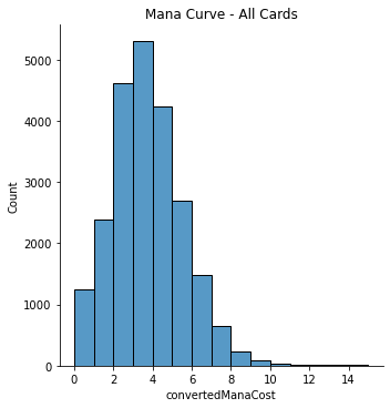
Insight:
- Overall, CMC for all cards shows that the mean is 3.29. The interquartile range of the box plot showing the middle 50% of scores results in 2 manas. This is calculated as Q3 or the upper quartile value of 4.0 minus the Q1 lower quartile value of 2.0.
CMC per Card Color
Checking if there is a null value in the convertedManaCost column.
print(df_cmc['convertedManaCost'].isna().sum())

# Creating new dataframe on each color
df_cmc_white = df_cmc[df_cmc["colors"]== 'White']
df_cmc_blue = df_cmc[df_cmc["colors"]== 'Blue']
df_cmc_black = df_cmc[df_cmc["colors"]== 'Black']
df_cmc_red = df_cmc[df_cmc["colors"]== 'Red']
df_cmc_green = df_cmc[df_cmc["colors"]== 'Green']
df_cmc_colorless = df_cmc[df_cmc["colors"]== 'Colorless']
df_cmc_multicolor = df_cmc[df_cmc["colors"]== 'Multicolor']

# Plot
x = [df_cmc_white['convertedManaCost'].tolist(),
     df_cmc_blue['convertedManaCost'].tolist(),
     df_cmc_black['convertedManaCost'].tolist(),
     df_cmc_red['convertedManaCost'].tolist(),
     df_cmc_green['convertedManaCost'].tolist(),
     df_cmc_colorless['convertedManaCost'].tolist(),
     df_cmc_multicolor['convertedManaCost'].tolist()]
plt.boxplot(x, labels=list(color_map.keys()))
plt.title('Converted Mana Cost per Card Color')
plt.ylabel('Converted Mana Cost')
plt.xlabel('Card Color')
plt.show()
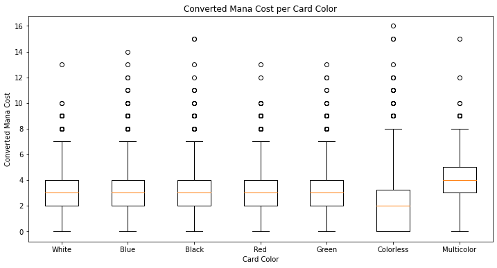
Insights:
- The mean CMC is located between 3-4 in all the colors. However, the
Whitecards have the lowest mean CMC, while theMulticolorcards have the highest mean CMC. When talking about speed, this makes theWhitecards one of the “fastest” colors in the game. - The interquartile range in all the cards is two manas, except for the
Multicolorcards. This indicates that the CMC distribution is centralized and consistent across the colors mentioned above. - Although all the colors have a similar CMC distribution in most of their cards, the outliers are the key difference between the “fast” colors (
RedandWhite) and the rest. - The
Whiteand theRedcards are the colors with the least number of outliers. This is probably the cause of their relatively low mean CMC.
CMC per Card Type
# Creating new dataframe on each type
df_cmc_creature = df_cmc[df_cmc["types"]== 'Creature']
df_cmc_instant = df_cmc[df_cmc["types"]== 'Instant']
df_cmc_enchantment = df_cmc[df_cmc["types"]== 'Enchantment']
df_cmc_sorcery = df_cmc[df_cmc["types"]== 'Sorcery']
df_cmc_artifact = df_cmc[df_cmc["types"]== 'Artifact']
df_cmc_others = df_cmc[df_cmc["types"]== 'Others']
df_cmc_land = df_cmc[df_cmc["types"]== 'Land']
df_cmc_planeswalker = df_cmc[df_cmc["types"]== 'Planeswalker']

# Plot
x = [df_cmc_creature['convertedManaCost'].tolist(),
     df_cmc_instant['convertedManaCost'].tolist(),
     df_cmc_enchantment['convertedManaCost'].tolist(),
     df_cmc_sorcery['convertedManaCost'].tolist(),
     df_cmc_artifact['convertedManaCost'].tolist(),
     df_cmc_others['convertedManaCost'].tolist(),
     df_cmc_land['convertedManaCost'].tolist(),
     df_cmc_planeswalker['convertedManaCost'].tolist()]
plt.boxplot(x, labels=list(df_sql['types'].unique()))
plt.title('Converted Mana Cost per Card Type')
plt.ylabel('Converted Mana Cost')
plt.xlabel('Card Type')
plt.show()
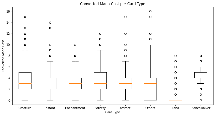
Insights:
Landcards can’t have a mana cost, as they are the mana’s main source.- The
CreatureandSorcerycards have a higher CMC. - The
Instantcards have the smallest interquartile range and the highest number of outliers, which makes them the most versatile card type.
Keywords (Abilities) Analysis
Overall Keywords
Double strike keywords are also considered as First strike. Therefore we need to change Double strike in the data to be counted as First strike.
print(f"First strike count: {df_sql['keywords'].value_counts()['First strike']}")

df_keywords = df_sql.copy()
df_keywords.loc[df_keywords['keywords'] == 'Double strike',
                'keywords'] = 'First strike'
print(f"First strike count: {df_keywords['keywords'].value_counts()['First strike']}")

keywords_cnt = df_keywords['keywords'].value_counts()[['Flying', 'First strike', 'Haste', 'Trample']]
keywords_cnt.plot(kind='bar')
plt.xticks(rotation=0, horizontalalignment="center")
plt.title('Popular Keywords of All Cards')
plt.xlabel('Card Keywords')
plt.ylabel('Card Count')
plt.show()
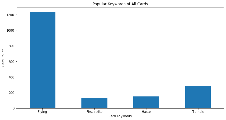
Insight:
- Overall
keywordsshow thatFlyinghas the highest count, followed by the ffkeywords(abilities) in decreasing order:Trample,Haste,First strike.
Keywords per Card Color
df_keywords_colors = pd.crosstab(df_keywords['colors'], df_keywords['keywords']).reindex(list(color_map.keys()))
display(df_keywords_colors.head())

pop_keyword = ['Flying', 'First strike', 'Haste', 'Trample']
df_keywords_colors[pop_keyword]

# Plot
for keyword in pop_keyword:
    df_keywords_colors[keyword].plot(kind='bar', color=list(color_map.values()))
    plt.xticks(rotation=0, horizontalalignment="center")
    plt.title(f'{keyword} type per Card Color')
    plt.xlabel('Card Color')
    plt.ylabel(f'Card Count of {keyword} type')
    plt.show()
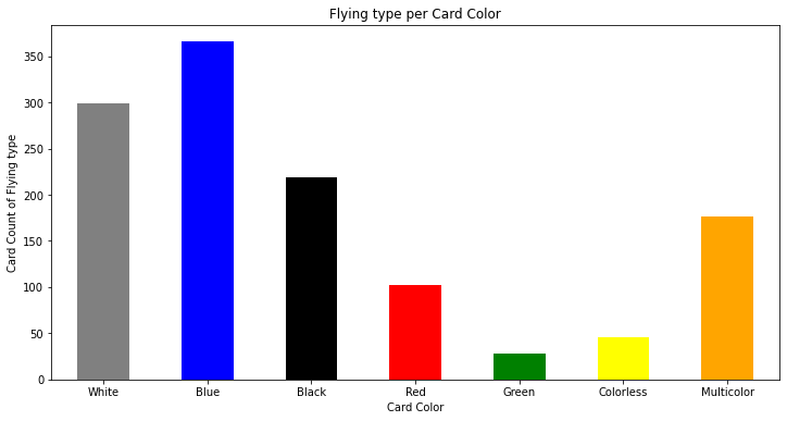
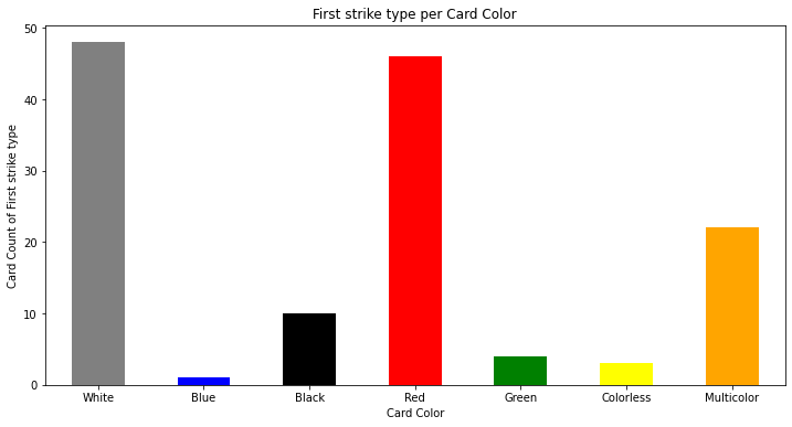
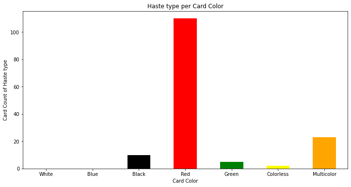
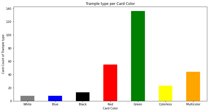
Insights:
BlueandWhitecreature cards have the highest count of theFlyingability. Although this may indicate favor towards these colors, tactics based on using all abilities, e.g.,Flying,First strike, etc., will determine a great strategy.RedandWhitecards have the highest occurrences ofFirst strike.Redcreatures have the highestHasteability count.GreenandRedcreatures have the highest occurrences ofTrample.
Elder Dragon Highlander Recommendations (EDHREC) Ranking Analysis
MTG has different game formats and rules of play. However, players were only bound to play compatible decks - until Adam Staley invented the Elder Dragon Highlander (EDH) Format. EDH was eventually adapted by MTG’s publisher, Wizards of the Cost, and sold Commander decks starting in 2011. Commander is a format in which you choose 100 cards; each of these cards — save for the lands — must be unique.
In this casual, multiplayer format, a player chooses a legendary creature to serve as the Commander and builds the rest of the deck around their color identity and unique abilities. Players are only allowed one of each card in their deck, except for basic lands, but they can use cards from throughout Magic’s history.
Every card in the Commander deck must only use mana symbols that also appear on the Commander. Colorless cards are allowed as well.
EDHREC is a crowdsourced repository of Commander decks and ideas – users submit decks, and EDHREC runs the numbers to tell you which cards are most popular in various lists.
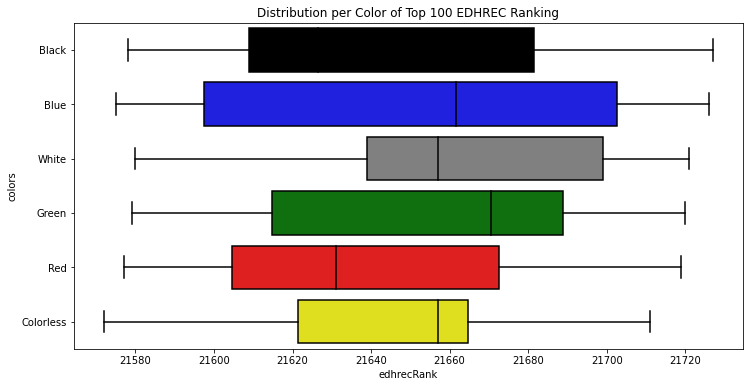
Below is a visualization of the Top 100 Most Popular Cards in EDH or Commander decks.
df_edh = df_sql.sort_values(by='edhrecRank', ascending=False)
df_edh_100 = df_edh.head(100)
sns_palette = [color_map[key] for key in list(df_edh_100['colors'].unique())]
sns.boxplot(data=df_edh_100, x='edhrecRank', y='colors', palette=sns_palette)
plt.title('Distribution per Color of Top 100 EDHREC Ranking')
plt.show()
sns.countplot(data=df_edh_100, y="colors", palette=sns_palette)
plt.title('Count per Color of Top 100 EDHREC Ranking')
plt.show()
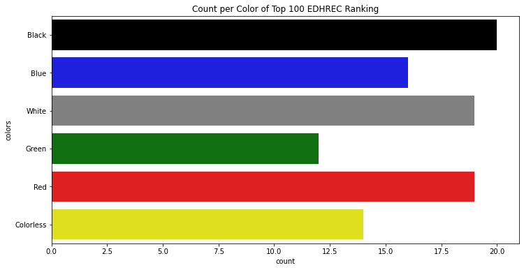
Insights:
Whiteflies over and ahead of the pack in popularity in the Commander/EDH Decks - both in frequency and ranking. However, no evidence suggests that such popularity results in or translates to any compelling winning advantage in MTG.Black,Red, andWhiteare most represented in the Top 100 EDHREC Ranking.Blue,White, andGreenenjoy high-rank scores.
Printings Analysis
color_printings = df_sql.groupby('colors')['printings'].sum()
print_colors = [color_map[key] for key in list(color_printings.index)]

# Plot
color_printings.plot(kind='bar', color=print_colors)
plt.xticks(rotation=0, horizontalalignment="center")
plt.title('Total No. of Reprintings per Card Color')
plt.xlabel('Card Color')
plt.ylabel('Printings Count ')
plt.show()
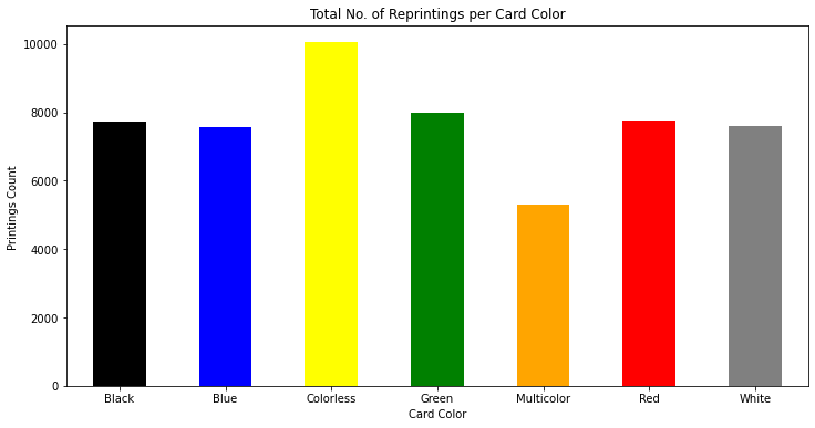
Insights:
Colorlessis the highest becauseLandcards are reprinted the most and areColorless.- All colors are printed fairly even.
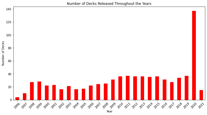
Deck Analysis
Deck List
df_decklist['year'] = pd.to_datetime(df_decklist['releaseDate']).dt.year
df_decklist = df_decklist.sort_values(by='releaseDate')
df_decklist = df_decklist.drop_duplicates(subset=['name'])
display(df_decklist.head())

# Plot
df_decklist['year'].value_counts(sort=False).plot(kind='bar', color='red')
plt.title('Number of Decks Released Throughout the Years')
plt.xticks(rotation=45, horizontalalignment="center")
plt.xlabel('Year')
plt.ylabel('Number of Decks')
plt.show()
print('The first deck was released in 1996.')
print('The year with the highest number of decks released is 2020 with',
      df_decklist['year'].value_counts().max(), 'decks.')
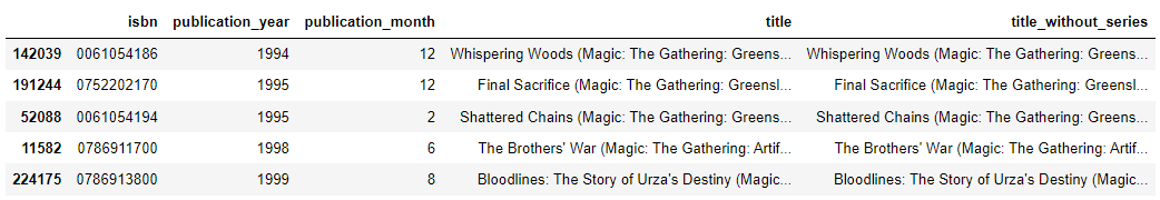
Books Connection (GoodReads)
# Removes rows with blank publication_year
df_books.drop(df_books[df_books['publication_year'] == ''].index,
              inplace=True)

# Filters Magic and The Gathering
df_books = df_books[(df_books['title']
                     .str.contains('magic', regex=False, case=False))
                    & (df_books['title']
                       .str.contains('the gathering',
                                     regex=False, case=False))]

# Sort by publication year
df_books = df_books.sort_values(by='publication_year')
df_books = df_books.drop_duplicates(subset=['title'])
df_books['publication_year'] = pd.to_datetime(df_books['publication_year'],
                                              format='%Y').dt.year

display(df_books.head())
Deck and Book Release
# Count number of decks/books per year
df_books_year = df_books['publication_year'].value_counts(sort=False)
df_decklist_year = (df_decklist['year'].value_counts(sort=False)
                    .rename("All_decks"))
df_decklist_year_th = (df_decklist.year[df_decklist['type'] == 'Theme Deck']
                       .value_counts(sort=False)).rename("Theme_decks")

df1 = pd.concat([df_books_year, df_decklist_year, df_decklist_year_th],
                axis=1)
df1 = (df1.sort_index().reset_index()
       .rename(columns={'index': 'Year', 'publication_year': 'Books'}))
year_list = df1.loc[:22, 'Year']
books_list = df1.loc[:22, 'Books']
alldecks_list = df1.loc[:22, 'All_decks']
themedecks_list = df1.loc[:22, 'Theme_decks']
display(df1.head())

# Create figure and axis #1 and Plot bar chart on axis #1
fig, ax1 = plt.subplots()
ax1.bar(year_list, alldecks_list, color='red')
ax1.set_ylabel('decks released')
ax1.legend(['Decks released'], loc="upper left")

# Set up the 2nd axis and Plot line chart on axis #2
ax2 = ax1.twinx()
ax2.plot(year_list, books_list, color='blue')
ax2.grid(False)  # turn off grid #2
ax2.set_ylabel('books')
ax2.legend(['Books published'], loc="upper right")
plt.title('No. of Decks Released vs. No. of Books Published that '
          'contains \nMagic: The Gathering (from 1994 to 2016)')
ax1.set_xlabel('Year')
plt.show()
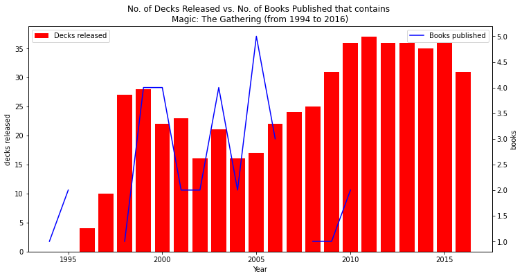
Insight:
- We look into the relationship of the decks released versus the number of books published that contain “Magic: The Gathering”. There seems to be no pattern within the two except for the years 2002 to 2004.
# Create figure and axis #1 and Plot bar chart on axis #1
fig, ax1 = plt.subplots()
ax1.bar(year_list, themedecks_list, color='red')
ax1.set_ylabel('decks released')
ax1.legend(['Theme decks released'], loc="upper left")

# Set up the 2nd axis and Plot line chart on axis #2
ax2 = ax1.twinx()
ax2.plot(year_list, books_list, color='blue')
ax2.grid(False) # turn off grid #2
ax2.set_ylabel('books')
ax2.legend(['Books published'], loc="upper right")
plt.title('No. of Theme Decks Released vs. No. of Books Published that '
          'contains \nMagic: The Gathering (from 1994 to 2016)')
ax1.set_xlabel('Year')
plt.show()
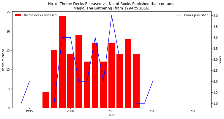
Insight:
- Looking deeper into the relationship of books published and the decks released, we discovered that Theme Decks contribute most in all of the decks released between 1999 to 2006. When the number of Theme Decks released went up in 1999, 2003, and 2005, the books published that contains the title “Magic: The Gathering” also increased.
Results
| Dataset | White | Blue | Black | Red | Green |
|---|---|---|---|---|---|
| Power | 1 | 2 | 3 | 4 | 5 |
| Toughness | 3 | 4 | 2 | 1 | 5 |
| CMC | 5 | 3 | 1 | 4 | 2 |
| Keywords: Flying | 4 | 5 | 3 | 2 | 1 |
| Keywords: First strike | 5 | 1 | 3 | 4 | 2 |
| Keywords: Haste | 1 | 2 | 4 | 5 | 3 |
| Keywords: Trample | 1 | 2 | 3 | 4 | 5 |
| EDHREC High Rank | 4 | 5 | 2 | 1 | 3 |
| EDHREC Frequency | 4 | 2 | 5 | 3 | 1 |
| Printings | 2 | 1 | 3 | 4 | 5 |
| Total | 30 | 27 | 29 | 32 | 32 |
Note: Colors are ranked from 1 to 5, with 5 being the highest. Magic: The Gathering can be seen as a very complex game. In different aspects, you can excel and simultaneously lose some advantages. The game continues to create and print new cards, which helps ensure the game is balanced.
It is also notable that cards with high power and toughness statistics, even having some unique skills, are only sometimes chosen by the players to be part of their deck. As evident from the EDHREC ranking and frequency of usage, any card is valuable and complements each other. The bottom line now is how one strategizes, plays the game, and maximizes the potential of each card.
Conclusion
Regardless of which Magic: The Gathering color the players choose, they all take on an equal opportunity to win. Each player is in for a metaphysical battle abundant in lore, challenges, and abilities.
It is in the players’ interest to carry on exploring and leveling up their gaming experience.
How a player moves from the equal position to the winning position requires strategy, timing, and excellent execution - dealing damage, decking, and playing on card advantage.
Players do not win by what color they play but by how they play Magic the Gathering.
References
[1] Churchill, A., S., B., & A., H. (2019). Magic: The Gathering is Turing Complete. Retrieved October 25, 2022 from https://arxiv.org/abs/1904.09828
[2] Cavotta, M. (2018, March 27). VENTURING OUTWARD WITH THE NEW MAGIC LOGO. Retrieved October 25, 2022 from Magic The Gathering: https://magic.wizards.com/en/articles/archive/news/venturing-outward-new-magic-logo-2018-03-27
[3] Emerging Technology from the arXiv. (2019, May 7). Magic: The Gathering” is officially the world’s most complex game. Retrieved October 25, 2022 from MIT Technology Review: https://www.technologyreview.com/2019/05/07/135482/magic-the-gathering-is-officially-the-worlds-most-complex-game/
[4] Hayes, J.S. (2019, Jun 12) A beginners guide to ‘Magic: the Gathering’ [Video]. Youtube. Retrieved October 25, 2022 from https://www.youtube.com/watch?v=8YNbo_SRUwY
[5] z80Wolfeh08z (2014, Sep 15) Magic The Gathering Cover Photo [Online Image]. Deviant Art. Retrieved October 25, 2022 from https://www.deviantart.com/z80wolfeh08z/art/Magic-The-Gathering-Cover-Photo-482404436
[6] thiagoam2 (2019, Sep 11) Nature Promise [Online Image]. Reddit. Retrieved October 25, 2022 from https://www.reddit.com/r/magicTCG/comments/d2d4pe/i_painted_a_card_and_want_to_know_what_you_think/
[7] Magic: The Gathering (n.d.) MTG Fandom. Retrieved October 25, 2022 from https://mtg.fandom.com/wiki/Magic:_The_Gathering
[8] [Magic: The Gathering Cards]. Magic The Gathering. Retrieved October 25, 2022 from https://magic.wizards.com/en
ACKNOWLEDGEMENT
I completed this project with my Sub Learning Team, which consisted of Felipe Garcia Jr. and Vanessa delos Santos.